Test of Difference

Author

Dr. Mohammad Nasir Abdullah

Test of Means Difference

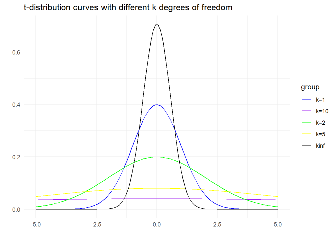
In this chapter, we will focus on test of difference in Parametric case and Non-Parametric case. The examples of Parametric test of difference are Independent t-test, Paired t-test, and One-Way Analysis of Variances. However, there are a lot more statistical technique for testing the difference of the variables. We limit the scope of this chapter in focusing on mentioned techniques. Of course the requirement of Parametric test of difference is Normality distributed data. If the Normality distribution assumption is violated, we may choose the alternative methods such as Non-Parametric test of difference. The Non-Parametric tests of difference that we will focus are Mann-Whitney test, Wilcoxon Sign Rank test, and Kruskal Wallis test.

t-test

Learning Objectives

After completing this topic, you should be able to understand the difference between parametric test and non-parametric test. Next, you should be able to determine when to use, the assumptions, and the steps in performing independent t-test and paired sample t-test. Furthermore, you should be able to interpret, present, make report, and conclusion from the analysis of independent sample t-test and paired sample t-test.

Introduction

The t-test is the most widely used method to evaluate the differences in mean between groups. The t-test and Analysis of Variance (ANOVA) are the parametric tests because they estimate parameters of some underlying normal distribution. The parametric test is usually being said to estimate at least one population parameter from sample statistics.

The main assumption for parametric test is the variable measured in the sample must be Normally Distributed in the population we plan to generalized our findings. The advantages of parametric test are it is more powerful and flexible methods and it allow researchers to study the effects of many variables and their interaction. While the disadvantages of the parametric test are the data can be seriously distorted by small number of sample and before the existence of the statistical software, it was very difficult to calculate.

Parametric tests like the t-test are preferred for their power and flexibility, especially in analyzing the effects of various variables and their interactions. However, their reliance on assumptions like normality and homogeneity of variance can be limiting. This is particularly true in cases of small or skewed samples, where these assumptions are violated.

In such scenarios, non-parametric tests become invaluable. These tests do not require the assumption of normal distribution, making them more suitable for ordinal data or when normality is not present. Common non-parametric counterparts to the t-test include the Mann-Whitney U test for independent samples and the Wilcoxon signed-rank test for paired samples. While less powerful than parametric tests when their assumptions are met, non-parametric tests offer robustness and reliability in the face of data that defy these assumptions.

This note aims to provide a comprehensive understanding of the t-test, its applications, and its limitations. Additionally, we will briefly explore non-parametric tests, understanding their role as alternatives to the t-test. This approach ensures a well-rounded comprehension of statistical analysis, equipping the reader with the knowledge to choose the appropriate test based on the nature of their data and research requirements.

T Distribution

Students’ t-distribution or simply said as the t-distribution is a probability distribution that arises in the problem of estimating the mean of a normally distributed population when the sample size is small. The Student’s t-distribution takes a single parameter which is the number of degrees of freedom of the sample. The probability curve of t-distribution looks like a normal distribution because as the number of degrees of freedom increase, this distribution approaches the normal distribution.

Warning: package 'ggplot2' was built under R version 4.3.2

In probability and statistics, the t-distribution is a probability distribution that arises in the problem of estimating the mean of a normally distributed population when the sample size is small. It is the basis of the popular Student’s t-test for the statistical significance of the difference between two sample means and for confidence interval for the difference between two population means.

Independent sample t-test

The independent sample t-test is a two sample test of the null hypothesis when the means of two normally distributed populations are equal. The objectives of this test are:

To compare the means of a numerical variable in two independent samples, or,
To determine whether the differences between the two observed mean exceeds the difference that would be expected by chance, or
To determine whether the difference between means of the two sets of the numerical variable is significant.

The most important part before starting to employed independent sample t-test is to make sure the dependent variable from independent sample is numerical.

Assumption of Independent sample t-test

There are five (5) assumptions need to be complied before performing and establishing the independent t-test, which are:

The dependent variable or the test variable must be numerical.
The sample is drawn randomly from the population of interest.
The observations should be independent (independent sample). This means that the sampling unit should appear in only one group (sampling unit should not be related or measured twice).
Normally assumption - means that the distribution of the data for each group must be normally distributed .
- If the data are more than or equal to 30, normality is assumed based on agreeable central limit theorem.
- If the data are less than 30, we should check the normality distribution using histogram, boxplot, etc.
Both groups should have the same variance (homogeneity of variance).

To Note!

The assumptions number 1 until 3 should be done at study design and sampling method stages.

Type of data requirement

Two types of data required for the analysis of independent sample t-test.

One independent variable. Should be in categorical variable with only 2 levels. For example: Intervention group and control group, male group and female group, Alzheimer’s patient and Health control subject.
One dependent variable. Should be in continuous variable. For example: Students’ score, PEFR score, and Weight.

Data for example

In this example, we will use penguins dataset from palmerpenguins library and mtcars dataset.

Steps in Independent sample t-test

There are five (5) steps in analysis of independent sample t-test:

State the hypothesis
Checking the assumptions
Performing R codes
Interpreting and conclusion
Presentation of the result

Example 1 : Penguins dataset

In this example, we want to know is there any difference on mean bill length, bill depth and flipper length between male and female penguins for Adelie Species

Research question:

1) Is the mean bill length significantly difference between male and female Adelie penguins?
2) Is the mean bill depth significantly difference between male and female Adelie penguins?
3) Is the mean flipper length significantly difference between male and female Adelie penguins?

Null Hypothesis

1) There is no significant difference on mean bill lengths between male and female Adelie penguins.
2) There is no significant difference on mean bill depth between male and female Adelie penguins.
3) There is no significant difference on mean flipper lengths between male and female Adelie penguins.

Checking Assumptions

1) There are 1 dependent variable and 1 independent variable:

Dependent variable (numerical): Bill Length (mm);
Independent variable (categorical with 2 levels): Sex (male and female)

2) The sample are independent (not related) and drawn out randomly.

3) Normality check:

library(tidyverse)
library(palmerpenguins)
library(nortest)

#Selecting only Adelie Species
Adelie <- penguins %>%
            drop_na() %>%
            filter(species == "Adelie")


#split the dataset into male and female
male_Adelie <- Adelie %>%
                     filter(sex == "male")

female_Adelie <- Adelie %>%
                     filter(sex == "female")


#Testing  the normality using lilliefors test
lillie.test(male_Adelie$bill_length_mm)


    Lilliefors (Kolmogorov-Smirnov) normality test

data:  male_Adelie$bill_length_mm
D = 0.070914, p-value = 0.484

lillie.test(female_Adelie$bill_length_mm)


    Lilliefors (Kolmogorov-Smirnov) normality test

data:  female_Adelie$bill_length_mm
D = 0.074018, p-value = 0.4143

Based on the Lilliefors test, we can conclude that the distribution of bill length for male [D-statistic: 0.070914, p-value: 0.4840] and female [D-statistic: 0.074018, p-value: 0.4143] are normally distributed since the p-value for male group was less than 0.05 .

Graphical presentation:

Male <- ggplot(male_Adelie, aes(bill_length_mm)) + 
  geom_histogram(bins = round(1+log2(length(Adelie$bill_length_mm))),
                 bg="lightblue", col="lightblue4") + 
  theme_minimal() +
  labs(title  = "Distribution of Bill Length \n for Male Adelie Penguins",
       x = "Bill Length in mm", 
       y = "Frequency") + 
  theme(plot.title = element_text(hjust=0.5, size = 9))


Female <- ggplot(female_Adelie, aes(bill_length_mm)) + 
  geom_histogram(bins = round(1+log2(length(Adelie$bill_length_mm))),
                 bg="lightpink", col="lightpink4") + 
  theme_minimal() +
  labs(title  = "Distribution of Bill Length \n for Female Adelie Penguins",
       x = "Bill Length in mm", 
       y = "Frequency") + 
  theme(plot.title = element_text(hjust=0.5, size = 9))


library(gridExtra)
grid.arrange(Male, Female, ncol=2,
             top="Histogram showing distribution of Bill Length for Male and Female Adelie Penguins")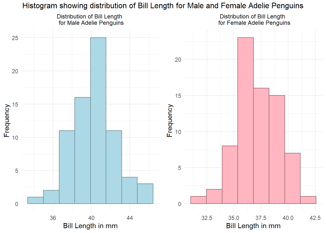

Based on the histogram, we can conclude that the bill length for male and female Adelie penguins were approximately normal distributed.

4) Checking homogeneity of variances

library(car)

Loading required package: carData


Attaching package: 'car'

The following object is masked from 'package:dplyr':

    recode

The following object is masked from 'package:purrr':

    some

leveneTest(Adelie$bill_length_mm~Adelie$sex, center = mean)

Levene's Test for Homogeneity of Variance (center = mean)
       Df F value Pr(>F)
group   1  0.2138 0.6445
      144

Null Hypothesis: The variances are equal for both groups
Alternative Hypothesis: The variances are not equal for both groups.

Based on the Levene’s Test for Homogeneity of variance, the p-value was more than 0.05, which concludes that the variance are equal for both groups [F-Statistic (df1, df2): 0.2138 (1,144), p-value: 0.6445].

Since all the assumptions for conducting independent sample t-test were met, now we can proceed with performing the test.

Performing Independent sample t-test

The t.test() function in R can be used for conducting an independent t-test, which is a statistical test used to compare the means of two independent groups. This test can be applied to data in both wide and long formats. Understanding the format of your data is crucial for correctly applying the t.test() function.

1. Independent t-test with Wide Format Data:

In wide format, each group’s data is in its own column. This is common when each group or condition is a separate column in your dataset.

Example of Wide Format Data:

  Group1  Group2
    2.3     2.8
    2.4     3.0
    2.5     2.9

How to Use t.test() with Wide Format Data: In this case, you simply pass the two columns (groups) into the t.test() function as separate arguments.

Syntax:

t.test(data$Group1, data$Group2, var.equal = TRUE)

2. Independent t-test with Long Format Data:

In long format, all values are in a single column, and another column indicates the group to which each value belongs. This format is common in datasets where multiple measurements are stacked in one column and another column indicates the category or group.

Example of Long Format Data:

  Value  Group
    2.3      1
    2.4      1
    2.5      1
    2.8      2
    3.0      2
    2.9      2

How to Use t.test() with Long Format Data: For long format data, you first need to subset the data into two vectors based on the group, and then pass these vectors to the t.test() function.

Syntax:

t.test(Value~Group, var.equal=TRUE)

Bill length and Sex

To perform the independent sample t-test to find the difference on mean bill length between male and female Adelie penguins, we noticed that from the assumption checking, the variances are equal for both group male and female, thus on the argument var.equal we will change it to TRUE (default = FALSE).

#Performing Independent sample t-test with equal variance assumed
t.test(Adelie$bill_length_mm~Adelie$sex, var.equal=TRUE)


    Two Sample t-test

data:  Adelie$bill_length_mm by Adelie$sex
t = -8.7765, df = 144, p-value = 4.44e-15
alternative hypothesis: true difference in means between group female and group male is not equal to 0
95 percent confidence interval:
 -3.838435 -2.427319
sample estimates:
mean in group female   mean in group male 
            37.25753             40.39041

#Display the mean and standard deviation for each group
Adelie %>%
  group_by(sex) %>%
  summarise(mean_length = mean(bill_length_mm),
            sd_length = sd(bill_length_mm))

# A tibble: 2 × 3
  sex    mean_length sd_length
  <fct>        <dbl>     <dbl>
1 female        37.3      2.03
2 male          40.4      2.28

Based on the independent sample t-test, we can conclude that there are significant difference on mean bill length between male and female Adelie penguins since the p-value was less than 0.05 [t-statistic (df): -8.7765 (144), p-value: <0.001]. Furthermore, the mean bill length for male [mean(sd): 40.39 (2.28)] longer compared to female [mean(sd): 37.26 (2.03)] penguins for Adelie species.

Presentation of the Results

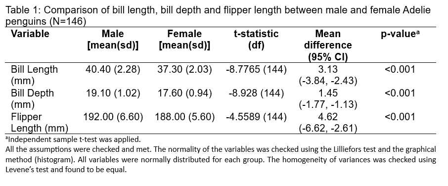
Assume that we already perform the independent sample t-test for bill length, bill depth and flipper length for male and female Adelie penguins. Now, we need to present the results into a statistical table to make a report.

Constructive reporting:

In a comparative study of the morphological characteristics of Adelie penguins, the dimorphism between males and females was analyzed using an independent sample t-test. The study encompassed a sample of 146 penguins and measured three variables: bill length, bill depth, and flipper length. Preliminary checks ensured the data met the assumptions required for t-testing; the normality of the variables was confirmed through the Lilliefors test and histogram analysis, and the homogeneity of variances was established using Levene’s test, ensuring the appropriateness of the subsequent statistical analysis.

The results indicated significant differences between males and females in all three measured characteristics. Males exhibited a longer bill length (mean = 40.40 mm, SD = 2.28 mm) compared to females (mean = 37.30 mm, SD = 2.03 mm), with a mean difference of 3.13 mm and a 95% confidence interval from -3.84 to -2.43. The bill depth followed a similar pattern, with males having a greater mean bill depth (mean = 19.10 mm, SD = 1.02 mm) than females (mean = 17.60 mm, SD = 0.94 mm) and a mean difference of 1.45 mm (95% CI: -1.77 to -1.13). Flipper length also differed, with male penguins having longer flippers (mean = 192.00 mm, SD = 6.60 mm) than females (mean = 188.00 mm, SD = 5.60 mm), and a mean difference of 4.62 mm (95% CI: -6.62 to -2.61). The t-statistics for bill length, bill depth, and flipper length were -8.7765, -8.928, and -4.5589, respectively, all with 144 degrees of freedom. The significant t-statistics and mean differences are supported by p-values less than 0.001, surpassing the conventional alpha level of 0.05, thus confirming the statistical significance of the differences.

The study unequivocally demonstrates sexual dimorphism in Adelie penguins, with male penguins showing consistently larger dimensions in bill length, bill depth, and flipper length compared to female penguins. These findings contribute valuable insights into the sexual selection and ecological adaptation of Adelie penguins. The high statistical significance of the results reinforces the reliability of the observed differences in physical characteristics between the sexes, potentially linked to differing roles in foraging and breeding behaviors. This research not only enhances our understanding of Adelie penguin biology but also aids in the broader context of avian ecological studies.

Example 2: `mtcars` dataset

In this example, mtcars dataset are used to demonstrate the different scenario in performing independent sample t-test when the equality of variance is not met.

Research Question: Is there any significant difference on mean Miles per Gallon between Automatic transmission and Manual transmission

Hypothesis: There is no significant difference on mean Miles per Gallon between Automatic transmission and Manual transmission

1) Load the dataset

data1 <- mtcars

#change am to factor variable
data1$am <- as.factor(data1$am)

2) Checking Normality Assumption on estimate by variable.

#selecting the rent group and income group
Manual <- data1 %>%
  drop_na() %>%
  filter(am == 1)

Automatic <- data1 %>%
  drop_na() %>%
  filter(am == 0)


#Normality test on Miles per Gallon for Automatic transmission cars
library(nortest)
lillie.test(Automatic$mpg)


    Lilliefors (Kolmogorov-Smirnov) normality test

data:  Automatic$mpg
D = 0.087337, p-value = 0.9648

#Normality test on Miles per Gallon for Manual transmission cars
lillie.test(Manual$mpg)


    Lilliefors (Kolmogorov-Smirnov) normality test

data:  Manual$mpg
D = 0.14779, p-value = 0.6107

Based on the Lilliefors test, both groups shows normally distributed Miles per Gallons.

3) Checking the homogeneity of variances

library(car)
leveneTest(data1$mpg~data1$am, center=mean)

Levene's Test for Homogeneity of Variance (center = mean)
      Df F value  Pr(>F)  
group  1   5.921 0.02113 *
      30                  
---
Signif. codes:  0 '***' 0.001 '**' 0.01 '*' 0.05 '.' 0.1 ' ' 1

Based on the Levene’s test, the p-value was less than 0.05, indicating that the variance for both group is not equal.

4) Performing independent sample t-test

t.test(data1$mpg~data1$am, var.equal=FALSE)


    Welch Two Sample t-test

data:  data1$mpg by data1$am
t = -3.7671, df = 18.332, p-value = 0.001374
alternative hypothesis: true difference in means between group 0 and group 1 is not equal to 0
95 percent confidence interval:
 -11.280194  -3.209684
sample estimates:
mean in group 0 mean in group 1 
       17.14737        24.39231

Based on the independent sample t-test, the p-value indicated value less than 0.05 [t-statistic(df): -3.76 (18.332), p-value: 0.0014]. It was found that there are statistically significant difference on mean Miles per Gallon between Automatic transmission and Manual Transmission.

5) Presentation of Results

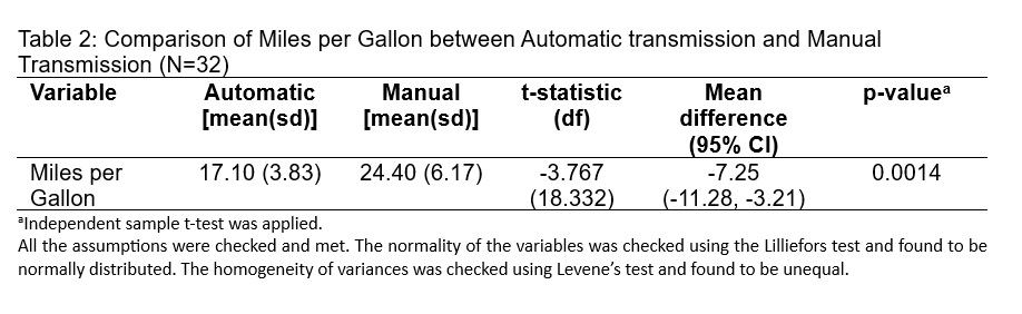
The results from Table 2 show a comparison of fuel efficiency, measured in miles per gallon (MPG), between vehicles with automatic transmission and those with manual transmission. The study included 32 vehicles. On average, cars with manual transmission achieved better fuel efficiency (24.40 MPG) than those with automatic transmission (17.10 MPG), with a mean difference of 7.25 MPG. The standard deviations indicate some variability within each group (3.83 MPG for automatic and 6.17 MPG for manual).

The t-statistic is -3.767, with 18.332 degrees of freedom, indicating that the difference in MPG is statistically significant, as shown by a p-value of 0.0014. This p-value is well below the typical threshold of 0.05, suggesting that the observed difference in MPG between transmission types is unlikely to have occurred by chance. It should be noted, however, that the variances between the two groups are unequal, as determined by Levene’s test. Despite this, the significant t-statistic suggests a genuine difference in fuel efficiency between the two transmission types.

Example 3: Example data from wide format

In this example, we will use wide format dataset to perform independent sample t-test.

1) lets reshape the dataset set from long format to wide format. using sleep dataset from base package.

# the original format
head(sleep)

  extra group ID
1   0.7     1  1
2  -1.6     1  2
3  -0.2     1  3
4  -1.2     1  4
5  -0.1     1  5
6   3.4     1  6

tail(sleep)

   extra group ID
15  -0.1     2  5
16   4.4     2  6
17   5.5     2  7
18   1.6     2  8
19   4.6     2  9
20   3.4     2 10

#reshape this data to wide format
sleep2 <- reshape(sleep, direction = "wide", 
                  idvar = "ID", timevar = "group")
head(sleep2)

  ID extra.1 extra.2
1  1     0.7     1.9
2  2    -1.6     0.8
3  3    -0.2     1.1
4  4    -1.2     0.1
5  5    -0.1    -0.1
6  6     3.4     4.4

In this reshaped dataset, we split the extra variable (hours of sleep) into two column representing extra.1 for drug 1 group, and extra.2 for drug 2 group.

Assuming the normality assumption is met and the equality of variance is met. The independent sample t-test is:

t.test(sleep2$extra.1, sleep2$extra.2, var.equal = TRUE)


    Two Sample t-test

data:  sleep2$extra.1 and sleep2$extra.2
t = -1.8608, df = 18, p-value = 0.07919
alternative hypothesis: true difference in means is not equal to 0
95 percent confidence interval:
 -3.363874  0.203874
sample estimates:
mean of x mean of y 
     0.75      2.33

The reporting scheme are same as before.

Exercise

1) Perform Independent sample t-test for bill length, bill depth and flipper length for male and female Gentoo penguins

2) using BMI.sav datafile from https://sta334.s3.ap-southeast-1.amazonaws.com/data/BMI.sav,
Does the mean BMI differ between Hypertension (HPT) and non-HPT group? Run Hypothesis testing and conclude your findings, take level of significance at 0.05.

3) Using HPT.sav datafile from https://sta334.s3.ap-southeast-1.amazonaws.com/data/hpt.sav,
Does the mean body mass index (BMI) differs between male and female in the study?

Paired Sample t-test

The paired sample t-test or matched sample t-test or related sample t-test is a test to find the difference of the two samples that are dependent or related. It is used when the data is from only one group of samples with two time measurement. Studies which employ a pre-test and post-test design may consider the paired sample t-test for the analysis. In the pre-test and post-test design, we measured the same variable twice, or maybe at two different time points and we are interested in whether this measure has changed in the duration. In addition, we may also have a separate group but they have been pair-wise matched in some way, this is also an example of paired sample t-test data. The most important part in the paired sample t-test is normally distributed data because this is under parametric test. An example of research design that can employ paired sample t-test is single arm pre and post-test study design as displayed below:

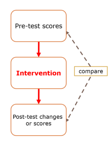
The research questions example for single arm pre and post-test are:

1) Is there any significant increase from pre-test to post-test score among the students after remedial class?
2) Is there any change in the thickness or arterial plaque before and after treatment with the vitamin E?

Assumption of Paired sample t-test

There are four (4) main assumptions need to be complied before proceeding with the analysis of paired t-test which are:

There are 2 test variables and it is numerical or continuous.
The data is gathered at random (means must gather using probabilistic sampling).
The observations or measurements are dependent or paired or matched.
The difference between paired data must be normally distributed.

Data Requirement

Since the paired t-test is measuring two points of dependent data, there is no independent variable. The two variables to be tested must be numerical or continuous.

Data Example

The obesity_paired_data.sav will be used to demonstrate on Paired sample t-test. The data can be downloaded from https://sta334.s3.ap-southeast-1.amazonaws.com/data/obesity_paired+data.sav

library(haven)
data1 <- read_sav("https://sta334.s3.ap-southeast-1.amazonaws.com/data/obesity_paired+data.sav")

head(data1)

# A tibble: 6 × 3
     ID BMIPRE BMIPOST
  <dbl>  <dbl>   <dbl>
1     1     25      22
2     2     23      21
3     3     20      21
4     4     26      22
5     5     21      20
6     6     26      23

Research Question
Is there any difference in Body Mass Index (BMI) among the randomly selected 60 participants after exercise intervention given?

Hypothesis
There is no significant difference on mean BMI before and after intervention.

Checking Assumption

1) checking normality of the difference between before and after intervention

#creating new variable (difference before and after)
data1$diff <- data1$BMIPRE-data1$BMIPOST

#performing lilliefors test 
library(nortest)
lillie.test(data1$diff)


    Lilliefors (Kolmogorov-Smirnov) normality test

data:  data1$diff
D = 0.0917, p-value = 0.2392

Based on the statistical test for normallity distribution using Lilliefors test, it was found that the difference BMI between before and after intervention was normally distributed since the p-value of Lilliefors was more than 0.05 [D-statistic: 0.0917, p-value: 0.2392].

by graphical presentation

ggplot(data1, aes(diff)) + 
  geom_boxplot() + 
  scale_y_continuous(limits = c(-1,1)) + 
  theme_minimal() + 
  labs(title = "The distribution of difference between BMI before and After intervention", 
       x="difference before and after")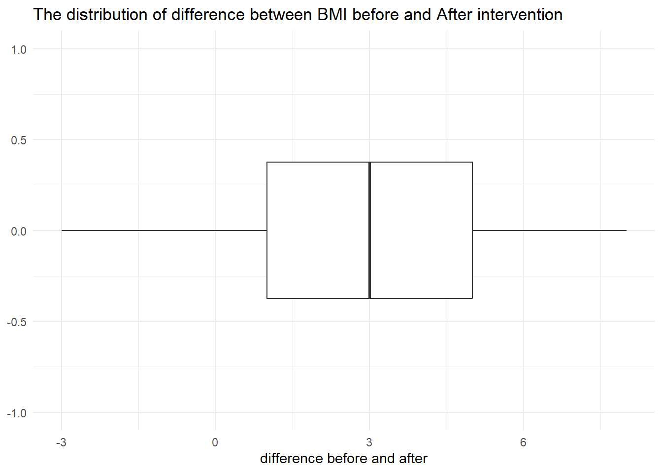

Based on the boxplot, it is clearly seen that the difference between BMI before and after was normally distributed.

Performing Paired Sample t-test

To perform Paired sample t-test, we use the same function as in independent sample test which is t.test(), but we will add another argument inside the function which is paired=TRUE.

t.test(data1$BMIPRE, data1$BMIPOST, paired=TRUE)


    Paired t-test

data:  data1$BMIPRE and data1$BMIPOST
t = 7.4724, df = 59, p-value = 4.283e-10
alternative hypothesis: true mean difference is not equal to 0
95 percent confidence interval:
 2.062406 3.570927
sample estimates:
mean difference 
       2.816667

Based on the result, we can conclude that there are significant difference on mean BMI before and after intervention since the p-value was less than 0.05 [t-statistic (df): 7.4724 (59), p-value: <0.001]. Futhermore, we can compare the effectiveness of the intervention by mean and standard deviation.

#mean
sapply(data1[-1], mean)

   BMIPRE   BMIPOST      diff 
24.483333 21.666667  2.816667

#standard deviation
sapply(data1[-1], sd)

  BMIPRE  BMIPOST     diff 
2.977268 1.684090 2.919784

Based on the mean, we can conclude that the mean BMI after [mean(sd): 21.67 (1.68)] intervention was improved compared to before [mean(sd): 24.48 (2.98)] intervention.

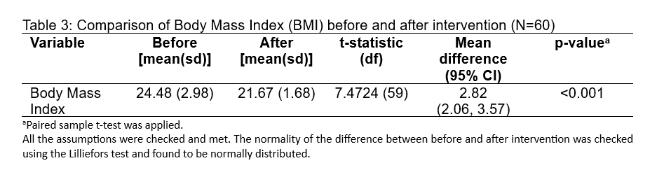
Reporting Paired sample t-test results

The table displays the results of a paired sample t-test comparing Body Mass Index (BMI) values before and after an intervention for a sample size of 60 (N=60). Here is how to interpret the results:

Mean BMI Before Intervention: The average BMI before the intervention was 24.48, with a standard deviation (sd) of 2.98. The standard deviation is a measure of the amount of variation or dispersion of a set of values.
Mean BMI After Intervention: The average BMI after the intervention was 21.67, with a standard deviation of 1.68. A smaller standard deviation indicates that the BMI values after the intervention were closer to the mean, suggesting less variability in BMI post-intervention.
t-Statistic: The t-statistic value is 7.4724. This is a measure of the difference between the two conditions in terms of the number of standard errors. A higher t-value indicates a greater degree of difference between the paired samples.
Degrees of Freedom (df): The degrees of freedom for this test is 59, which is calculated as the number of pairs (N) minus 1. This is used to determine the critical value of t from the t-distribution table, which in turn helps in calculating the p-value.
Mean Difference (95% CI): The mean difference between the pre- and post-intervention BMI is 2.82, and the 95% confidence interval (CI) for this mean difference is (2.06, 3.57). This means that we can be 95% confident that the true mean difference in the population from which the sample was drawn lies within this interval.
p-Value: The p-value is <0.001, which means that the probability of observing such a large mean difference (or larger) due to random chance, if there was actually no difference (null hypothesis is true), is less than 0.1%. Since this p-value is below the common alpha level of 0.05, the result is statistically significant, indicating strong evidence against the null hypothesis of no change.
Assumptions: The text below the table notes that all the assumptions for the paired sample t-test were checked and met, which includes the assumption of normality for the differences between pairs. The normality was confirmed using the Lilliefors test.

In summary, the table suggests that the intervention was effective in reducing BMI among the participants, with the reduction being statistically significant.

Exercise 2

An instructor wants to use two exams in her classes next year. This year, she gives both exams to the students. She wants to know if the exams are equally difficult and want to check this by looking at the differences between scores. If the mean difference between scores for students is “close enough” to zero, she will make a practical conclusion that the exams are equally difficult. Here the data:

   Student Exam_1_Score Exam_2_Score
1      Bob           63           69
2     Nina           65           65
3      Tim           56           62
4     Kate          100           91
5   Alonzo           88           78
6     Jose           83           87
7   Nikhil           77           79
8    Julia           92           88
9    Tohru           90           85
10 Michael           84           92
11    Jean           68           69
12   Indra           74           81
13   Susan           87           84
14   Allen           64           75
15    Paul           71           84
16  Edwina           88           82

One way Analysis of Variance (One-way ANOVA)

In the independent sample t-test, we can only compare between two groups. However, if we are interested in finding the difference of a numerical data among more than 2 groups, we are dealing with different combinations of pairs of means. If we use multiple independent t-test to compare different pair of means, we are at risk of increasing type 1 error. There is a perfect way to handle numerical data on comparing more than 2 groups, the analysis is called Analysis of Variance (ANOVA). It is called one-way because we are looking at the impact of only one independent variable on the dependent variable.

By mathematics, analysing the variability (variance) of groups can tell us whether their mean differ or otherwise. To determine whether the between-group difference is large enough to reject the null hypothesis, we compare it statistically to the within-group difference, based on F-test.

Where F is defined as variation among sample means divided by variation among individuals in same sample. In theory, the larger the overall F values, the more statistically significant it will be or in other word there is a mean difference between group.

Type of data required

Just like independent sample t-test, the One-way ANOVA also requires two type of variables:

1) One dependent variable (numerical/continuous). For example: age of the students, blood pressure, cholestrol levels.
2) One independent variable (categorical with more than 2 levels). For example: drug groups (Drug A, Drug B, Control), Teaching style (whole class, small group, self-paced).

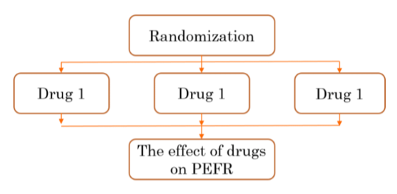
Example of Suitable Research Design

The analysis of variance (ANOVA) usually suitable for two types of research design such as experimental or randomized trial design and observational design. In an experimental design, the subject are assigned randomly to the different groups of interest and the difference of the effect are measured. For example, let say a pharmacist dispensed drugs for lung function to patients with asthma. Then, he or she wished to determined whether there are differences in mean Peak Expiratory Flow Rate (PEFR) among three different drug group (say: Drug 1, Drug 2, and Control). [ This example are taken from book published by Nyi Nyi Naing and Wan Arfah Nadiah, 2011].

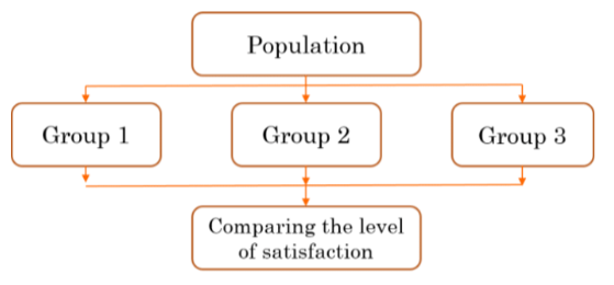
Another example is an observational study design. In an observational study (for example, cross sectional, etc..), the subjects defined their own groups after being recruited as a sampling unit. The easiest example is the comparison of average level of satisfaction among three different groups in the population.

Assumption for ANOVA

There are five assumptions for one-way ANOVA test which are:

The test variable must be numerical or continuous.
The data are taken using probabilistic sampling techniques (must be random).
The groups are independent of each another.
Each groups must comply the normality assumption.
Homogeneity of variance, which means that the variance for each group should be equal.

The assumptions number 2 and 3 should be settled at research design and sampling techniques stages.

Data for Example

In this example, we will use penguins dataset from palmerpenguins to compare bill length, bill depth and flipper length between species of penguins (Adelie, Chinstrap, and Gentoo).

Step to execute One-Way ANOVA

There are basically five steps to be comply for one-way ANOVA. Such steps are:

Hypothesis statement
Checking the assumptions
Perform one-way ANOVA
Interpretation
Presentation of the results

Research Question

Is there any significant difference on the mean bill length between three species of penguins (Adelie, Chinstrap, and Gentoo)?
Is there any significant difference on the mean bill depth between three species of penguins?
Is there any significant difference on the mean flipper length between three species of penguins?

Hypothesis:

Null Hypothesis: There is no significant difference on the mean bill length between three species of penguins.

Alternative Hypothesis: There is a significant difference on the mean bill length between three species of penguins.

Checking Assumptions

As mentioned previously, the assumptions of random sampling and independent data are determined by the study design and sampling design.

1) Checking Normality assumptions

#Separating the species into difference set
Adelie <- penguins %>%
  filter(species == "Adelie")
Chinstrap <- penguins %>%
  filter(species == "Chinstrap")
Gentoo <- penguins %>%
  filter(species == "Gentoo")

#checking normality for Adelie on bill Length
lillie.test(Adelie$bill_length_mm)


    Lilliefors (Kolmogorov-Smirnov) normality test

data:  Adelie$bill_length_mm
D = 0.042489, p-value = 0.7254

#checking normality for Chinstrap on bill Length
lillie.test(Chinstrap$bill_length_mm)


    Lilliefors (Kolmogorov-Smirnov) normality test

data:  Chinstrap$bill_length_mm
D = 0.093769, p-value = 0.1459

#checking normality for Gentoo on bill Length
lillie.test(Gentoo$bill_length_mm)


    Lilliefors (Kolmogorov-Smirnov) normality test

data:  Gentoo$bill_length_mm
D = 0.062001, p-value = 0.2929

Based on the normality analysis using Lilliefors test, we can conclude that there are normality distributed for bill length for Adelie penguins [D-Statistic: 0.0425, p-value: 0.7254], Chinstrap penguins [D-Statistic: 0.0938, p-value: 0.1459], and Gentoo penguins [D-Statistic: 0.062, p-value: 0.2929] since the p-value were more than 0.05.

2) Checking Homogeneity of Variances

The Levene’s test is used to check for homogeneity of variances.

library(car)
leveneTest(penguins$bill_length_mm~penguins$species, center=mean)

Levene's Test for Homogeneity of Variance (center = mean)
       Df F value  Pr(>F)  
group   2  2.8336 0.06019 .
      339                  
---
Signif. codes:  0 '***' 0.001 '**' 0.01 '*' 0.05 '.' 0.1 ' ' 1

Based on the Levene’s test of homogeneity of variances, we can conclude that the variances for all groups are equal since the p-value was more then 0.05 [F-statistic (df1, df2): 2.8336 (2, 339), p-value: 0.0602].

Performing one-way ANOVA

To perform one-way ANOVA, we can use aov() function.

fit <- aov(penguins$bill_length_mm~penguins$species)
summary(fit)

                  Df Sum Sq Mean Sq F value Pr(>F)    
penguins$species   2   7194    3597   410.6 <2e-16 ***
Residuals        339   2970       9                   
---
Signif. codes:  0 '***' 0.001 '**' 0.01 '*' 0.05 '.' 0.1 ' ' 1
2 observations deleted due to missingness

Based on the one-way ANOVA result, we can conclude that there is a significant difference on mean bill length between three species (Adelie, Chinstrap, and Gentoo) since the p-value was less than 0.05 [F-statistic (df1, df2): 410.60 (2, 339), p-value: <0.001]. Since there is a significant difference on mean bill length, we need to further investigate which species is differ in term of mean bill length. Thus, the post-hoc test need to be perform to determine the specific differences.

Since the homogeneity of variance assumption was met, we will use TukeyHSD test to perform the multiple comparison test.

To note: there are several methods to perform multiple comparisons for one-way ANOVA if the equality of variances assumed. The methods are not limited to TukeyHSD, but Bonferroni, Hommel, Benjamini & Yekutieli, Benjamini & Hochberg, and many more. If the equality of variances not assumed, The Games-Howell method, Hommel method and many more can be used to cater for multiple comparisons.

Multiple Comparison (Post-Hoc Test)

In this stage, we will use TukeyHSD method to perform multiple comparison, you can change it to others method such as Bonferroni etc..

TukeyHSD(fit)

  Tukey multiple comparisons of means
    95% family-wise confidence level

Fit: aov(formula = penguins$bill_length_mm ~ penguins$species)

$`penguins$species`
                      diff       lwr        upr     p adj
Chinstrap-Adelie 10.042433  9.024859 11.0600064 0.0000000
Gentoo-Adelie     8.713487  7.867194  9.5597807 0.0000000
Gentoo-Chinstrap -1.328945 -2.381868 -0.2760231 0.0088993

Based on the TukeyHSD method, we can conclude that there are significant difference on mean bill length between Chinstrap and Adelie [mean difference: 10.04, p-value: <0.001], Gentoo and Adelie [mean difference: 8.713, p-value: <0.001], and Gentoo and Chinstrap [mean difference: -1.329, p-value: 0.0089] since the p-value were less than 0.05.

To illustrate the difference, we can construct the mean plot to see the difference of the mean bill length between Adelie penguins, Chinstrap penguins and Gentoo penguins.

library(gplots)
  plotmeans(bill_length_mm ~ species, data = penguins,
            xlab = "Species", ylab = "Bill Length (mm)",
            main="Mean Plot with 95% CI")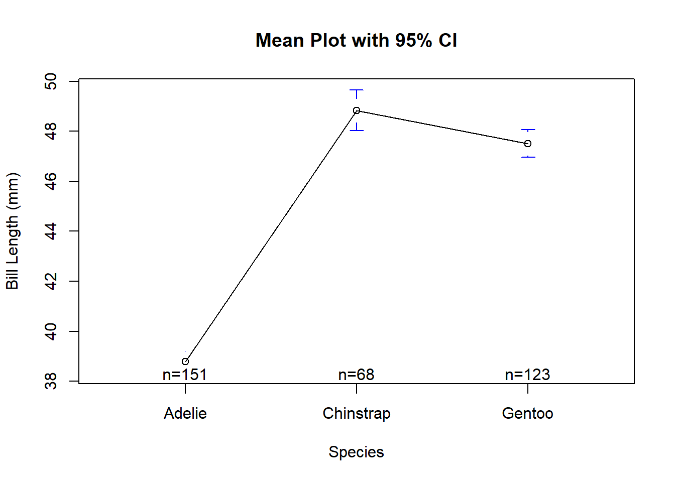

Based on the mean plot, we can conclude that the mean bill length has significantly difference between Adelie penguins and Gentoo penguins, Adelie penguins and Chinstrap penguins. However, there are slight difference on mean bill length between Chinstrap and Gentoo penguins.

Yet, another way to present mean plot :

 library(ggpubr)
  ggline(penguins, x = "species", y = "bill_length_mm", 
         add = c("mean_se", "jitter"), 
         order = c("Adelie", "Chinstrap", "Gentoo"),
         ylab = "Mean Bill Length (mm)", xlab = "Species")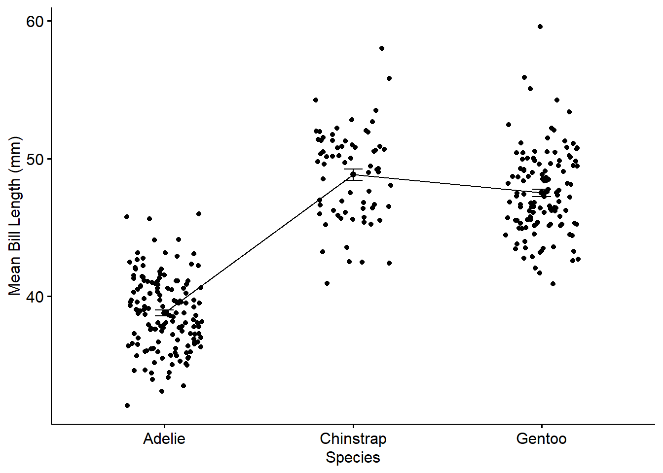

Reporting one-way ANOVA

#getting the mean and sd for each species
penguins %>%
  group_by(species) %>%
  summarise(n = n(), 
            mean1 = mean(bill_length_mm, na.rm=T),
            sd1 = sd(bill_length_mm, na.rm=T))

# A tibble: 3 × 4
  species       n mean1   sd1
  <fct>     <int> <dbl> <dbl>
1 Adelie      152  38.8  2.66
2 Chinstrap    68  48.8  3.34
3 Gentoo      124  47.5  3.08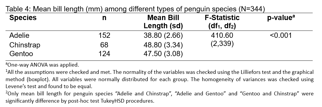

In a comparative analysis of the bill lengths among different penguin species, a one-way ANOVA was performed on a sample of 344 penguins across three distinct species: Adelie, Chinstrap, and Gentoo. The Adelie species, with a sample size of 152, exhibited a mean bill length of 38.80 mm with a standard deviation of 2.66 mm. In contrast, the Chinstrap and Gentoo species, with sample sizes of 68 and 124 respectively, displayed larger mean bill lengths of 48.80 mm (sd = 3.34 mm) and 47.50 mm (sd = 3.08 mm), respectively. The differences in bill length across the species were analyzed using an F-statistic of 410.60 with degrees of freedom (df1, df2) of (2,339), and a resulting p-value of less than 0.001, indicating a highly statistically significant difference in mean bill lengths across the species.

The robustness of the ANOVA results was underpinned by the confirmation of all test assumptions, including the normal distribution of bill lengths within each species group, as assessed by the Lilliefors test, and the homogeneity of variances confirmed by Levene’s test. To further explore the pairwise differences between the species’ mean bill lengths, a Tukey HSD post-hoc test was employed, revealing significant distinctions between each pair of species. The Adelie species’ mean bill length was significantly shorter than both the Chinstrap and Gentoo species, while the latter two also differed significantly from each other. This detailed analysis provides a clear indication of the morphological differences among the species, potentially contributing to our understanding of their ecological niches and feeding adaptations in the Palmer Archipelago of Antarctica.

Exercise 3

Continue to perform the one-way ANOVA for bill depth and flipper length to determine the significant difference between Adelie, Chinstrap and Gentoo penguins. Do all nessessary procedures. start with stating research questions, hypothesis, etc. What can you conclude from the analysis?
Using dataset Data Obesity Women_2009.sav, from https://sta334.s3.ap-southeast-1.amazonaws.com/data/Data+Obesity+Women_+2009.sav.

Question: An observational study to assess waist among randomly selected obesity patients data on their different BMI status: Underweight, Normal, Overweight, and Obese.

Research Question: Does the mean waist differ among obese patients who have different BMI status?

Test of Means Difference

t-test

Learning Objectives

Introduction

T Distribution

Independent sample t-test

Assumption of Independent sample t-test

Type of data requirement

Data for example

Steps in Independent sample t-test

Example 1 : Penguins dataset

Checking Assumptions

Performing Independent sample t-test

1. Independent t-test with Wide Format Data:

2. Independent t-test with Long Format Data:

Bill length and Sex

Presentation of the Results

Example 2: mtcars dataset

Example 3: Example data from wide format

Exercise

Paired Sample t-test

Assumption of Paired sample t-test

Data Requirement

Data Example

Checking Assumption

Performing Paired Sample t-test

Reporting Paired sample t-test results

Exercise 2

One way Analysis of Variance (One-way ANOVA)

Type of data required

Example of Suitable Research Design

Assumption for ANOVA

Data for Example

Step to execute One-Way ANOVA

Checking Assumptions

Performing one-way ANOVA

Multiple Comparison (Post-Hoc Test)

Reporting one-way ANOVA

Exercise 3

Example 2: `mtcars` dataset