The categorical data analysis has extensively been used in various areas to conclude their findings. Example of areas that frequently use the categorical data analysis include behavioural sciences, medical sciences, political philosophy, zoology, public health, marketing, education, and many more. Even some quantitative areas such as quality control and engineering also apply categorical data analysis when to classify items into a certain standards.
Categorical data analysis requires data to be categorical either the scales should be in nominal or ordinal. Usually the purpose of categorical data analysis is to find the association between categorical variables. One of the examples of research question is ” What are the factors associated with hypertension among men?“.
In this note, we will discuss thoroughly about categorical data analysis on Chi-squared and Fisher-Exact test.
In future, this note will be add more regarding McNemar test, Mantel Haenzal test, Kappa agreement test, odd ratio, relative risk, and Bland-Altman agreement test.
Contingency Table
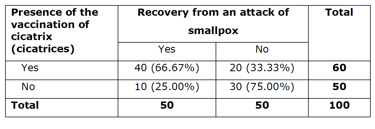
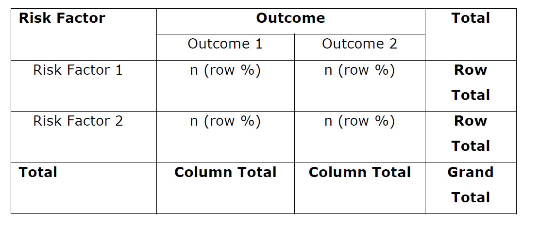
The contingency table is a cross tabulation of the categorical variables where each cell shows the value of each category in combination of two or more. The row of contingency table is for independent variable or risk factors or exposure whereas the column is for outcome of the study or dependent variable. The presentation of these tables is according to the matrix format. According to Pearson, the contingency table usually classify the two variables into a number of groups and in this manner, the table has been formed containing columns and rows compartment. The total frequency of the population under consideration is distributed into sub-groups corresponding to these rows and columns. An example of contingency table for presence of the vaccination cicatrices (vaccination of healing injured tissue) and the recovery from an attack of smallpox can be shown as table below:
Table 1: Tabulation of presence of the vaccination of cicatrix and recovery from an attack of smallpox (n=100)
As we can see from Table 1, two variables involved which are presence of the vaccination of cicatrices (yes and no) and recovery from an attack of smallpox (yes and no). The numbers inside the table are frequency count and percentage. To read these contingency table, out of 100 patients observed, we can summaries that there are 40 patients (66.67%) had taken the vaccination of cicatrices and had recovered from smallpox. Furthermore, there are 20 patients (33.33%) who had taken vaccination on cicatrices and did not recover from an attack of smallpox.
Apparently, we can summaries the general contingency table as below:
To extract or construct contingency table in R, let see the example from Fisher’s psychophysical experiment named as “Tea Taster” in his book titled The Design of Experiments (Fisher, 1974) which described that a Lady who declares herself can discriminate whether the milk or the tea mix first added to the cup.
The results shows that out of 8 cups of tea tasting by the lady, 3 cups are correctly guessed for milk and 1 cup is wrongly guessed for milk infusion, and same goes to tea infusion. As you can see on the result, on each row, there are 2 values, these values are number (upper side) and percentage (lower side). The percentage represents row percentage, which means that on “First Mixture on Milk”, there are 75% correct guessed “Yes” and the balance is 25% wrongly guessed. This experiment actually used 70 trials cups of tea for that lady to choose only 4 cups for each mixture.
Test of Independence for Contingency table
In this section, we will demonstrate some good tests to measure the association and difference between one, two or more categorical variables. The statistical test involved are one-way Chi-Squared test (Goodness of Fit Chi-Squared test), Pearson Chi-Squared test and Fisher’s Exact test where these test are appropriate for nominal data and the variables are independent to each other. The meaning of independent of each other is that two variables are not match sample or repeatedly measured.
One-way Chi-Squared Test
On having a single nominal categorical variable, the Chi-Squared analysis for one sample is the most appropriate test to measure difference and association between categories. These test often called as goodness of fit Chi-squared test. The main assumptions for this test are as follows:
1) The categorical variable should be in nominal scale.
2) Independent sample - which means that the respondents or observations cannot be measured more than once in the sample. This usually done at sampling techniques and study design.
3) Expected frequency less than 5 should not exceed 20%.
The purpose of doing this test is to find the difference between category levels on single nominal categorical variable. It compares between self-categories.
Example 1
Let’s look at data421.sav, (get this data via this link: https://sta334.s3.ap-southeast-1.amazonaws.com/data/data421.sav). This data contains only one nominal categorical variable which is education. The levels in this education variable are UPSR, PMR, SPM, STPM, Diploma, and Ijazah. Suppose we want to know is there any difference on these five highest education qualifications among respondents. The possible hypothesis are:
H0: The highest education qualifications among respondents are equal.
H1: The highest education qualifications among respondents are not equal.
Steps:
1) Lets load the dataset into R environment.
library(foreign)data1 <-read.spss("https://sta334.s3.ap-southeast-1.amazonaws.com/data/data421.sav", to.data.frame =TRUE)#To get the frequency tabletable(data1$Education, useNA="ifany")
Now, we can perform the one-way chi-square test or goodness of fit chi-square test to determine is there any significant association between the highest education. Before, we can conclude the analysis, we must note that, the expected value / expected frequency for each categories should be more than 5. If there are expected frequency less than 5, it should not more than 20% of the overall categories available.
performing the goodness of fit chi-square test / one-way chi-square test.
test <-chisq.test(table(data1$Education))#looking at the expected frequenciestest$expected
The residual shows a difference between observed value and expected value. The higher the residual will indicates higher discrepancy of the particular group.
The Chi-square result
print(test)
    Chi-squared test for given probabilities

data:  table(data1$Education)
X-squared = 126.29, df = 5, p-value < 2.2e-16
The Chi-Square value was 126.29 with 5 degree of freedom. These value are enough to indicate that it has a significant difference result. But in this note, we try to avoid any calculation, so we just look at the p-value. The p-value was less than 0.001.
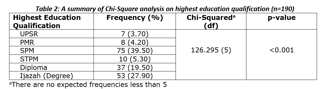
To report this result of the analysis, we need to construct a proper table and take important information from R output. The example of table for reporting purpose is as below:
Based on Table 2, we can conclude that at least one of the category levels of highest education qualification was statistically significantly different since the p-value was less than 0.001 (less than 0.05). Furthermore, it was found that most of the respondents have SPM as their highest education qualification (39.50%), it was followed by Degree (27.90%), and Diploma (19.50%). The least number of respondents with the highest education qualification is UPSR and PMR by 3.70% and 4.20% respectively.
G-Test
Another test could be useful to reconfirm the result above, is by using G test (the log likelihood ratio) goodness of fit test.
The G-test, or log-likelihood ratio test, is a statistical test used for assessing the goodness of fit between observed and expected frequencies in a contingency table. It is commonly employed when comparing the observed distribution of categorical data to an expected distribution, and it is particularly useful when sample sizes are small.
The test is based on the log-likelihood ratio, which measures how well the observed frequencies fit the expected frequencies. The formula for the G-test statistic is:
G = 2 * summation of Observed(i) * log(Observed(i) / Expected (i))
The test statistic G follows a chi-square distribution, and the degrees of freedom depend on the number of categories and constraints in the model. The formula for the degrees of freedom (df) is df=number of categories − number of parameters estimated.
The null hypothesis of the G-test is that there is no difference between the observed and expected frequencies, indicating a good fit. The alternative hypothesis suggests a significant difference, implying a poor fit.
library(DescTools) #this require R version>=4.3GTest(table(data1$Education))
    Log likelihood ratio (G-test) goodness of fit test

data:  table(data1$Education)
G = 129.25, X-squared df = 5, p-value < 2.2e-16
The interpretation are the same as goodness of fit Chi-Squared test.
Post-Hoc Test
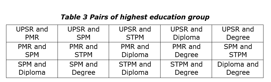
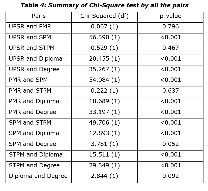
The result does not give detail information on which groups are different, it only gives general information indicating that there are at least one different group. Therefore, we need an additional test to confirm which groups are different and which are not. The next step basically the same step as above but with a bit of modification of the data selection. We need to compare by pairing the group. We need to test the difference between UPSR and PMR, UPSR and SPM, UPSR and STPM, and so on. In this case we will have 15 pairs to be tested. To do this, we need to identify the pairs that need to be analyse, this can be seen as table below:
To ensure we do not commit the type 1 error in concluding the finding, the alpha value should be adjusted by dividing to the number of pairs in comparison. For example, we take 0.05 as our benchmark alpha value, we then divided the value with 15 (which is the number of comparison pairs). The new alpha would be 0.05 / 15 = 0.0033. If the p-value less than 0.0033, we would conclude that there is a significant difference between the pairs.
Steps:
#UPSR and PMRa1 <- data1 %>%filter(Education %in%c("UPSR", "PMR")) %>%mutate(Education =droplevels(Education))chisq.test(table(a1))
    Chi-squared test for given probabilities

data:  table(a1)
X-squared = 0.066667, df = 1, p-value = 0.7963
    Chi-squared test for given probabilities

data:  table(a2)
X-squared = 56.39, df = 1, p-value = 5.942e-14
#UPSR and STPMa3 <- data1 %>%filter(Education %in%c("UPSR", "STPM")) %>%mutate(Education =droplevels(Education))chisq.test(table(a3))
    Chi-squared test for given probabilities

data:  table(a3)
X-squared = 0.52941, df = 1, p-value = 0.4669
#UPSR and Diplomaa4 <- data1 %>%filter(Education %in%c("UPSR", "Diploma")) %>%mutate(Education =droplevels(Education))chisq.test(table(a4))
    Chi-squared test for given probabilities

data:  table(a4)
X-squared = 20.455, df = 1, p-value = 6.106e-06
#UPSR and Degreea5 <- data1 %>%filter(Education %in%c("UPSR", "Ijazah")) %>%mutate(Education =droplevels(Education))chisq.test(table(a5))
    Chi-squared test for given probabilities

data:  table(a5)
X-squared = 35.267, df = 1, p-value = 2.875e-09
#PMR and SPMa6 <- data1 %>%filter(Education %in%c("PMR", "SPM")) %>%mutate(Education =droplevels(Education))chisq.test(table(a6))
    Chi-squared test for given probabilities

data:  table(a6)
X-squared = 54.084, df = 1, p-value = 1.921e-13
#PMR and STPMa7 <- data1 %>%filter(Education %in%c("PMR", "STPM")) %>%mutate(Education =droplevels(Education))chisq.test(table(a7))
    Chi-squared test for given probabilities

data:  table(a7)
X-squared = 0.22222, df = 1, p-value = 0.6374
#PMR and Diplomaa8 <- data1 %>%filter(Education %in%c("PMR", "Diploma")) %>%mutate(Education =droplevels(Education))chisq.test(table(a8))
    Chi-squared test for given probabilities

data:  table(a8)
X-squared = 18.689, df = 1, p-value = 1.539e-05
#PMR and Degreea9 <- data1 %>%filter(Education %in%c("PMR", "Ijazah")) %>%mutate(Education =droplevels(Education))chisq.test(table(a9))
    Chi-squared test for given probabilities

data:  table(a9)
X-squared = 33.197, df = 1, p-value = 8.329e-09
#SPM and STPMa10 <- data1 %>%filter(Education %in%c("SPM", "STPM")) %>%mutate(Education =droplevels(Education))chisq.test(table(a10))
    Chi-squared test for given probabilities

data:  table(a10)
X-squared = 49.706, df = 1, p-value = 1.786e-12
#SPM and Diplomaa11 <- data1 %>%filter(Education %in%c("SPM", "Diploma")) %>%mutate(Education =droplevels(Education))chisq.test(table(a11))
    Chi-squared test for given probabilities

data:  table(a11)
X-squared = 12.893, df = 1, p-value = 0.0003298
#SPM and Degreea12 <- data1 %>%filter(Education %in%c("SPM", "Ijazah")) %>%mutate(Education =droplevels(Education))chisq.test(table(a12))
    Chi-squared test for given probabilities

data:  table(a12)
X-squared = 3.7812, df = 1, p-value = 0.05183
#STPM and Diplomaa13 <- data1 %>%filter(Education %in%c("STPM", "Diploma")) %>%mutate(Education =droplevels(Education))chisq.test(table(a13))
    Chi-squared test for given probabilities

data:  table(a13)
X-squared = 15.511, df = 1, p-value = 8.204e-05
#STPM and Degreea14 <- data1 %>%filter(Education %in%c("STPM", "Ijazah")) %>%mutate(Education =droplevels(Education))chisq.test(table(a14))
    Chi-squared test for given probabilities

data:  table(a14)
X-squared = 29.349, df = 1, p-value = 6.044e-08
#Diploma and Degreea15 <- data1 %>%filter(Education %in%c("Diploma", "Ijazah")) %>%mutate(Education =droplevels(Education))chisq.test(table(a15))
    Chi-squared test for given probabilities

data:  table(a15)
X-squared = 2.8444, df = 1, p-value = 0.09169
The results can be presented as follows:
Table 4 shows that analysis by group pairs were done using one-way Chi-Square test as a follow up procedure after general one-way Chi-Square test to know which pair or group is different. The analysis shows that the expected frequencies less than 5 is none, thus the assumption of Chi-Squared is hold. We can conclude that at the p-value, only pairs of “UPSR and PMR”, “UPSR and STPM”, “PMR and STPM”, “SPM and Degree”, and “Diploma and Degree” have no statistically significant difference since the p-value for all these pairs are more than 0.0033.
Exercise 1
using library vcd, load the Suicide dataset. Please read the documentation of Suicide dataset.
1) Determine is there any significant association between the suicide methods in Germany (poison, cookgas, toxicgas, hang, drown, gun, knife, jump, and other). Present the results and make an appropriate interpretation for the results obtained.
Test of Independent (Pearson’s Chi-Squared test)
If you have two (2) independent nominal categorical variables, the Pearson Chi-Squared test of independence is appropriate test to measure the association and difference between two independent nominal variables for large sample size (Agresti, 2007). Theoretically, the Pearson’s Chi-Squared test came from Chi-Squared distribution. The Pearson Chi-Squared statistic formula to test on the null hypothesis is summation of (number of observed - number of expected) ^ 2 divided by the grant total.
This formula was proposed by Karl Pearson in 1900 who was an applied mathematician who completed Todhunter’s history of the theory of elasticity and later become one of the greate British Statistician (Plackett, 1983).
The purpose of the test is to find the difference and association between two independent categorical variables with nominal scales. To proceed with the test, all assumptions need to be comply with some conditions as stated below:
1) The subject or data must be independent and not related.
a. This can be settled during sampling techniques and study design.
2) The two (2) variables are categorical with nominal scale.
3) The expected count of less than 5 should be less than 20%.
Basically, if we want to test the association between two independent nominal variables, the example of research questions are :
1) Is gender associated with hypertension status?
2) Is gender associated with preferred breakfast?
#Important Notes
The Pearson’s Chi-Squared mainly caters for two categorical variables with nominal scale.
Example 1
We will use Hospital dataset from vcd library. The dataset represent table related to the length of stay (in years) of 132 long-term schizophrenic patients in two London mental hospitals with the frequency of visits.
Remember, this dataset was already made in contingency table.
#To see the datasetlibrary(vcd)
Loading required package: grid
Hospital
                   Length of stay
Visit frequency     2-9 10-19 20+
  Regular            43    16   3
  Less than monthly   6    11  10
  Never               9    18  16
We would test the variable visit frequency and length of stay, the research question is
Does the number of hospital visit concludes that the longer length of stay in hospital? or
Is the number of hospital visit associated with the length of stay in hospital?
The possible hypothesis is:
H0: Number of Hospital visit has no significant association with length of stay in hospital.
H1: Number of visit has significant association with length of stay in hospital.
or
H0: The number of hospital visit does not related to the length of stay in the hospital.
H1: The number of hospital visit does related with the length of stay in the hospital.
Performing the Chi-Square test of Independent
To perform the Chi-square test of independent, the best way is to use the gmodel library if we only have one pair to compare.
                   Length of stay
Visit frequency          2-9     10-19       20+
  Regular           27.24242 21.136364 13.621212
  Less than monthly 11.86364  9.204545  5.931818
  Never             18.89394 14.659091  9.446970
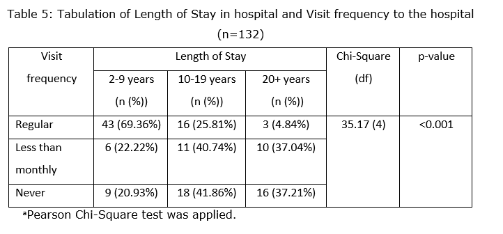
Based on the result, there are 9 cells combined (3 categories for visit frequency and 3 categories for length of stay). The expected value (expected frequency) for all cells were more than 5. It means that there are 0% of cells that having expected value less than 5. Thus, we can proceed with Pearson’s Chi-Squared analysis to conclude the association between length of stay in hospital and frequency hospital visit. The final result can be presented as below:
Based on Table 5, the total of 132 patients were included in the analysis. We found that out of 58 patients who stay in the hospital in 2 to 9 years, 43 patients (69.36%) were did regular visit to the hospital, 6 patients (22.22%) visit less than monthly, and 9 patients (20.93%) never visit the hospital. Next, out of 45 patients who stay in the hospital in 10 to 19 years, 16 patients (25.81%) were regular visitor, 11 patients (40.74%) visit less than monthly, and 18 patients (41.86%) never visit the hospital. For patients who stayed in the hospital more than 20 years, 3 patients (4.84%) were regular visitors, 10 patients (37.04%) visit less than monthly, and 16 patients (41.86%) never visit the hospitals. Furthermore, based on the Pearson’s Chi-square analysis, we found that the length of stay in the hospital and visit frequency to the hospital were statistically significant associated since the p-value was less than 0.05 [Chi-Squared (df): 35.17 (4); p-value < 0.001]. Overall, we can conclude that the longer the length of stay in hospital, the less frequent the visits.
#Gender and lifestylelibrary(gmodels)CrossTable(table(cereals$active, cereals$gender), format ="SPSS", prop.c =FALSE, prop.t =FALSE,prop.chisq =FALSE, expected =TRUE, chisq =TRUE)
   Cell Contents
|-------------------------|
|                   Count |
|         Expected Values |
|             Row Percent |
|-------------------------|

Total Observations in Table:  880

             |
             |     Male  |   Female  | Row Total |
-------------|-----------|-----------|-----------|
    Inactive |      236  |      238  |      474  |
             |  228.382  |  245.618  |           |
             |   49.789% |   50.211% |   53.864% |
-------------|-----------|-----------|-----------|
      Active |      188  |      218  |      406  |
             |  195.618  |  210.382  |           |
             |   46.305% |   53.695% |   46.136% |
-------------|-----------|-----------|-----------|
Column Total |      424  |      456  |      880  |
-------------|-----------|-----------|-----------|


Statistics for All Table Factors


Pearson's Chi-squared test
------------------------------------------------------------
Chi^2 =  1.062957     d.f. =  1     p =  0.3025418

Pearson's Chi-squared test with Yates' continuity correction
------------------------------------------------------------
Chi^2 =  0.9280067     d.f. =  1     p =  0.3353814


       Minimum expected frequency: 195.6182
Step 3: Checking the assumptions
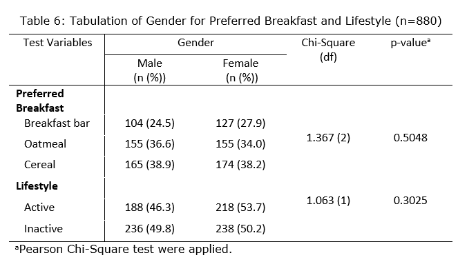
For testing the association between gender and preferred breakfast, there were 6 cells available for breakfast (3) and gender (2) categories. The expected value for each cells were more than 5, which met the assumption required to perform Pearson’s Chi-square test. For testing the association between gender and lifestyle, there were 4 cells available for lifestyle (2) and gender (2) categories. The expected value for each cells were more than 5, which also met the assumption required to perform Pearson’s Chi-square test.
Step 4: Presenting the result
Based on Table 6, There’s no statistically significant association between gender and preferred breakfast type (p-value = 0.5048) [Chi-Square (df): 1.367 (1)]. However, the percentages suggest a slight tendency for women to prefer breakfast bars more often than men (27.9% vs 24.5%). Similarly, there’s no significant association between gender and lifestyle (active vs inactive) based on the chi-square test (p-value = 0.3025) [Chi-Square (df): 1.063 (1)]. The percentages show a slightly higher proportion of women reporting an active lifestyle compared to men (53.7% vs 46.3%). The results suggest that gender might not be a strong predictor of breakfast preferences or lifestyle choices within this particular sample.
Exercise 2
1) Consider the penguins dataset, which includes information about different penguin species. Investigate the association between the variables “Species” and “Island” using Pearson’s Chi-square test. Provide the appropriate R code and interpret the results.
2) Explore the relationship between the variables “Sex” and “Species” in the penguins dataset using Pearson’s Chi-square test. Write R code to perform the analysis and discuss the findings in the context of the penguin dataset.
Fisher’s Exact Test
Fisher’s Exact test is a statistical test used to determine if there are non-random association between two categorical variables in a 2x2 contingency table. It is an exact test, meaning the results are not affected by the sample size. It is particularly useful when the sample sizes are small, and you cannot use the Chi-Square test.
When to use Fisher’s Exact test?
Use Fisher’s Exact test when:
You have two categorical variable
The data is in 2x2 contingency table
The sample size is small
Expected frequency of the cells in the contingency table are less than 5 more than 20%
Conducting the Fisher’s Exact test
To conduct the Fisher’s Exact test, follow these steps:
1) Formulate the null hypothesis (H0) that there is no association between the two categorical variables.
2) Construct a 2x2 contingency table to observe the frequency distribution of the categories.
3) Use the fisher.test() function in R to perform the test.
4) Determine the p-value from the test output.
5) Reject the null hypothesis if the p-value is less than the chosen significant level (usually 0.05).
Warning in chisq.test(t, correct = TRUE, ...): Chi-squared approximation may be
incorrect
Warning in chisq.test(t, correct = FALSE, ...): Chi-squared approximation may
be incorrect
   Cell Contents
|-------------------------|
|                   Count |
|         Expected Values |
|             Row Percent |
|-------------------------|

Total Observations in Table:  126

             |
             | known hpt  |   non hpt  | Row Total |
-------------|-----------|-----------|-----------|
       malay |       28  |       92  |      120  |
             |   29.524  |   90.476  |           |
             |   23.333% |   76.667% |   95.238% |
-------------|-----------|-----------|-----------|
   non-malay |        3  |        3  |        6  |
             |    1.476  |    4.524  |           |
             |   50.000% |   50.000% |    4.762% |
-------------|-----------|-----------|-----------|
Column Total |       31  |       95  |      126  |
-------------|-----------|-----------|-----------|


Statistics for All Table Factors


Pearson's Chi-squared test
------------------------------------------------------------
Chi^2 =  2.19056     d.f. =  1     p =  0.1388588

Pearson's Chi-squared test with Yates' continuity correction
------------------------------------------------------------
Chi^2 =  0.988854     d.f. =  1     p =  0.3200226


Fisher's Exact Test for Count Data
------------------------------------------------------------
Sample estimate odds ratio:  0.3079056

Alternative hypothesis: true odds ratio is not equal to 1
p =  0.1582781
95% confidence interval:  0.03900138 2.428276

Alternative hypothesis: true odds ratio is less than 1
p =  0.1582781
95% confidence interval:  0 1.791211

Alternative hypothesis: true odds ratio is greater than 1
p =  0.9680479
95% confidence interval:  0.05286802 Inf


       Minimum expected frequency: 1.47619
Cells with Expected Frequency < 5: 2 of 4 (50%)
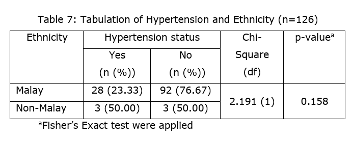
Based on the results, there were 4 cells combined for race and hypertension status. The expected values (expected frequency) for non-malay categories were less than 5 for known hpt and non-hpt which 1.476 and 4.524 respectively. Based on this, we can calculate the percentage of cells that having expected value less than 5, which is 2/4 * 100% = 50% (this is more than 20% allowable minimum expected values). This result can be seen at the bottom of the result “Cells with Expected Frequency < 5: 2 of 4 (50%)”.
3) Example how to report the result
Based on Table 7, out of a total of 126 patients, we found that the Malay patients (28 patients) with hypertension were higher compared to non-Malays (3 patients). For non-hypertension, the total of Malay patients were 92 and the rest are Non-Malay. Furthermore, we can conclude that there were no association between Ethnicity and Hypertension status since the Fisher’s Exact test p-value is 0.158 which is larger than 0.05 [Chi-Square (df): 2.191 (1)].
Example 2
Let’s use the mtcars dataset to perform the Fisher’s Exact test. In this example, we will test the association between the transmission type (am: 0=automatic, 1=manual), and the number of cylinders (cyl) in the car. Since cyl has more than two categories, we will recode it into two categories: 4 cylinders and not 4 cylinders.
Research Question: Is there any association between transmission type and number of cylinders?
Hypothesis: There are significant association between transmission type and number of cylinders.
Steps:
1) Load mtcars and recode the number of cylinders into 2 categories
data1 <- mtcars#Recode the 'cyl' variable into two categories: 4 and not 4data1$cyl_recode <-ifelse(data1$cyl ==4, '4', 'not 4')#convert cyl and am variable to factor variablesdata1$am <-as.factor(data1$am)data1$cyl_recode <-as.factor(data1$cyl_recode)
2) Create contingency table and hence perform Chi-Square test
Warning in chisq.test(t, correct = TRUE, ...): Chi-squared approximation may be
incorrect
Warning in chisq.test(t, correct = FALSE, ...): Chi-squared approximation may
be incorrect
   Cell Contents
|-------------------------|
|                   Count |
|         Expected Values |
|             Row Percent |
|-------------------------|

Total Observations in Table:  32

             |
             |        4  |    not 4  | Row Total |
-------------|-----------|-----------|-----------|
           0 |        3  |       16  |       19  |
             |    6.531  |   12.469  |           |
             |   15.789% |   84.211% |   59.375% |
-------------|-----------|-----------|-----------|
           1 |        8  |        5  |       13  |
             |    4.469  |    8.531  |           |
             |   61.538% |   38.462% |   40.625% |
-------------|-----------|-----------|-----------|
Column Total |       11  |       21  |       32  |
-------------|-----------|-----------|-----------|


Statistics for All Table Factors


Pearson's Chi-squared test
------------------------------------------------------------
Chi^2 =  7.1614     d.f. =  1     p =  0.007448904

Pearson's Chi-squared test with Yates' continuity correction
------------------------------------------------------------
Chi^2 =  5.276969     d.f. =  1     p =  0.02160934


Fisher's Exact Test for Count Data
------------------------------------------------------------
Sample estimate odds ratio:  0.1271682

Alternative hypothesis: true odds ratio is not equal to 1
p =  0.0205494
95% confidence interval:  0.01530014 0.7790805

Alternative hypothesis: true odds ratio is less than 1
p =  0.01065596
95% confidence interval:  0 0.6188523

Alternative hypothesis: true odds ratio is greater than 1
p =  0.9990097
95% confidence interval:  0.02100384 Inf


       Minimum expected frequency: 4.46875
Cells with Expected Frequency < 5: 1 of 4 (25%)
In this example, we can see that there are one cell that having expected value less than 5. This means that there are 25% of the total cells having expected value less than 5. This violated the assumption of Pearson’s Chi-Squared. Hence, we will proceed with Fisher’s Exact test.
The presentation of the result is same as previous.
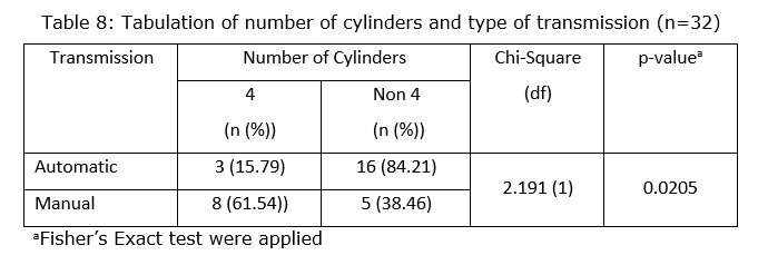
Based on Table 8, test of association between number of cylinders and type of transmission for 32 cars was performed. Out of 32 cars, there are 11 cars with 4 cylinders, from these 4 cars (15.79%) having automatic transmission and 8 cars (61.54%) having manual transmission. Next, there were 21 cars with non 4 cylinders, from these 16 cars (84.21%) having automatic transmission and 5 cars (38.46%) having manual transmission. Furthermore, we can conclude that there is an association between number of cylinders and type of transmission since the p-value for Fisher’s Exact test was less than 0.05 [Chi-Square (df): 2.191 (1); p-value: 0.0205].
Exercise 3
1) Investigate whether there is a significant association between the categorical variable “gear” and the binary variable “am” (automatic/manual transmission) in the mtcars dataset using Fisher’s Exact test. Provide the R code and explain the implications of the analysis.
2) Consider hpt.sav dataset from this link: https://sta334.s3.ap-southeast-1.amazonaws.com/data/hpt2.sav. Test the association between variable ethnicity and hpt, ethnicity and gender, ethnicity and bmicat. Provide the R code and explain the implications of the analysis.