#loading the dataset into R environment
library(haven)
data1 <- read_sav("https://sta334.s3.ap-southeast-1.amazonaws.com/data/patient+satisfaction.sav")Multiple Linear Regression
Multiple Linear Regression
Multiple linear regression (MLR) is the estimation of the linear relationship between a dependent variable and more than one independent variables or covariates. This analysis are applied in /exploratory studies and some in confirmatory studies, also not to forget an experimental situation where the experimenter can control the predictor variables. The example of multiple linear regression is to find the relationship between predictor variables (eg: age, weight, height) and the outcome variable (eg: PEFR (Peaked Exploratory Flow Rate)). If we are looking at relationship of individual independent variable to PEFR, it may not sound biologically. Therefore, we need to look at the relationship when all variables are considered at the same time towards the outcome PEFR. By doing this, we can look into presence of confounding and interactions.
In a nutshell, a single predictor or independent variable in the model would have provided an inadequate description since a number of key variables affect the outcome variable in important and distinctive ways. In addition, in situation of this type, we frequently find that predictions of the response variable based on a model containing only a single predictor variable, are too imprecise to be useful.
| Some Notation! |
|---|
|
Basic Theory
Model equation for multiple linear regression is expressed by the value of a predictand variable as a linear function of one or more predictor variables and an error term:
\[ Y = \beta_{0}+\beta_{1}X_{1}+\beta_{2}X_{2}+…+\beta_{n}X_{n}+e_{i} \]
where:
- Y is the outcome.
- Beta 0 is Y intercept
- B1 to Bn are the regression coefficient for individual independent variables.
- X1 to Xn are individual independent variables.
- e is an error term.
Our interest is in regression coefficient, its 95% confidence interval and corresponding p-value.
The model is estimated by least squares, which yields parameter estimates such that the sum of squares of errors is minimized. The error term is unknown because the true model is unknown. Once the model has been estimated, the regression residuals are defined as
\[ \overbrace{\epsilon} = y_{i}-\overbrace{y_{i}} \]
where yi is observed value of predictand for i observation. and Yi-hat is predicted value of predictand for i observation.
The residuals measure the closeness of fit of the predicted values and actual predictand in the calibration period. The algorithm for estimating the regression equation (solution of the normal equations) guarantees that the residuals have a mean of zero for the calibration period. The variance of the residuals measures the “size” of the error, and is small if the model fits the data well.
Assumption of Multiple Linear Regression
There are five assumptions that need to be met when performing multiple linear regression:
1) Linearity of the relationship between dependent and independent variables.
2) Statistical Independence of the errors (this should be settled during study design).
3) Homoscedasticity of the error (constant variance).
4) Normality of the error distribution.
5) Fit of independent numerical variable.
Types of data required
The type of data required for multiple linear regression are same as in simple linear regression. However, for independent variable, it should be more than one independent variables.
Steps in performing Multiple Linear Regression
1) Data exploration (descriptive statistics) and data cleaning.
2) Univariable analysis (Scatter plots and Simple Linear Regression).
3) Variable selection (Preliminary main-effect model)
4) Checking interaction and multicollinearity (Preliminary final model)
5) Checking model assumptions (Final Model)
***need remedial measures if problem are detected.
6) Interpretation and data presentation.
| Things to Note! |
|---|
| To perform Multiple Linear Regression, you need some knowledge from simple linear regression. Since we have discussed thoroughly in simple linear regression, the multiple linear regression would be more or less equal to the previous notes, thus the discussion in this section will be reduced. |
Example 1
In this example, we will use patient satisfaction.sav dataset from this link: https://sta334.s3.ap-southeast-1.amazonaws.com/data/patient+satisfaction.sav. The dataset is taken from a book titled “Applied Linear Statistical Model by Neter and Kutner (1996)”. The description of this example:
A hospital administrator wished to study the relation between patient satisfaction and patient’s age (years), severity of illness (index), and anxiety level (index). The administrator randomly select 46 patients and collected the data where the larger the value means more satisfaction, increased severity of illness and more anxiety.
Y = Patient satisfaction
X1 = Patient’s age in years
X2 = Severity illness (Index)
X3 = Anxiety level (index)
Research questions:
1) Is there any significant relationship between patient’s satisfaction and patient’s age?
2) Is there any significant relationship between patient’s satisfaction and severity illness?
3) Is there any significant relationship between patient’s satisfaction and anxiety level?
Hypothesis:
1) There are significant relationship between patient’s satisfaction and patient’s age.
2) There are significant relationship between patient’s satisfaction and severity illness.
3) There are significant relationship between patient’s satisfaction and anxiety level.
Research Question for multiple linear regression:
What are the factors contributed to patient’s satisfaction ?
or
How do patient age, severity of illness, and anxiety level collectively influence patient satisfaction in a hospital?
Hypothesis:
Null Hypothesis: There is no significant linear relationship between patient satisfaction and the combination of patient’s age, severity of illness, and anxiety level.
Alternative Hypothesis: There is a significant linear relationship between patient satisfaction and the combination of patient’s age, severity of illness, and anxiety level.
Step 1: Data exploration
Displaying first 6 observations
| Table 1: First 6 observations | |||
| Patient Satisfaction | Patient's Age (years) | Severity illness (Index) | Anxiety Level (index) |
|---|---|---|---|
| 48 | 50 | 51 | 2.3 |
| 57 | 36 | 46 | 2.3 |
| 66 | 40 | 48 | 2.2 |
| 70 | 41 | 44 | 1.8 |
| 89 | 28 | 43 | 1.8 |
| 36 | 49 | 54 | 2.9 |
Displaying some descriptive statistics:
# gtsummary
library(gtsummary)#StandWithUkrainemeansd <- data1 %>%
tbl_summary(
missing = "no",
statistic = list(all_continuous() ~ "{mean} ({sd})")) %>%
add_n() %>%
modify_header(label = "**Variables**",
all_stat_cols() ~ "**Mean (SD)**")
medianiqr <- data1 %>%
tbl_summary(
missing = "no",
statistic = list(all_continuous() ~ "{median} ({IQR})")) %>%
modify_header(label = "**Variables**",
all_stat_cols() ~ "**Median (IQR)**")
minmax <- data1 %>%
tbl_summary(
missing = "no",
statistic = list(all_continuous() ~ "{min} ({max})")
) %>%
modify_header(label = "**Variables**",
all_stat_cols() ~ "**Minimum (Maximum)**")
tbl_merge(
tbls = list(meansd, medianiqr, minmax),
tab_spanner = c("Measure 1", "Measure 2", "Measure 3")) %>%
modify_caption("Table 2: Descriptive statistics for all variables")| Variables | Measure 1 | Measure 2 | Measure 3 | |
|---|---|---|---|---|
| N | Mean (SD)1 | Median (IQR)2 | Minimum (Maximum)3 | |
| Patient Satisfaction | 46 | 62 (17) | 60 (29) | 26 (92) |
| Patient's Age (years) | 46 | 38 (9) | 38 (14) | 22 (55) |
| Severity illness (Index) | 46 | 50.4 (4.3) | 50.5 (5.0) | 41.0 (62.0) |
| Anxiety Level (index) | 46 | 2.29 (0.30) | 2.30 (0.38) | 1.80 (2.90) |
| 1 Mean (SD) | ||||
| 2 Median (IQR) | ||||
| 3 Minimum (Maximum) | ||||
Getting the scatter diagram for each dependent and independent variables.
library(ggplot2)
library(gridExtra)

#Satisfaction and Age
a <- ggplot(data1, aes(x=x1, y=Y)) +
  geom_point(size = 3, bg = "grey88", col="grey12", pch = 21) +
  geom_smooth(method = "lm", color="grey14",
              lwd = 0.5, lty = 2, se = F) +
  labs(title = "A Scatter plot showing relationship between \n Patient Satisfaction and Patient's Age (n=46)",
       x = "Patient's Age",
       y = "Patient Satisfaction") +
  theme_minimal() +
  theme(plot.title = element_text(hjust=0.5, size = 8))

#Satisfaction and Severity illness
b <- ggplot(data1, aes(x=x2, y=Y)) +
  geom_point(size = 3, bg = "grey88", col="grey12", pch = 21) +
  geom_smooth(method = "lm", color="grey14",
              lwd = 0.5, lty = 2, se = F) +
  labs(title = "A Scatter plot showing relationship between \n Patient Satisfaction and Severity illness (n=46)",
       x = "Severity illness",
       y = "Patient Satisfaction") +
  theme_minimal() +
  theme(plot.title = element_text(hjust=0.5, size = 8))

#Satisfaction and Anxeity Level
c <- ggplot(data1, aes(x=x3, y=Y)) +
  geom_point(size = 3, bg = "grey88", col="grey12", pch = 21) +
  geom_smooth(method = "lm", color="grey14",
              lwd = 0.5, lty = 2, se = F) +
  labs(title = "A Scatter plot showing relationship between \n Patient Satisfaction and Anxiety Level",
       x = "Anxiety Level",
       y = "Patient Satisfaction") +
  theme_minimal() +
  theme(plot.title = element_text(hjust=0.5, size = 8))

grid.arrange(arrangeGrob(a,b, ncol = 2),
             arrangeGrob(c, ncol = 1), nrow = 2)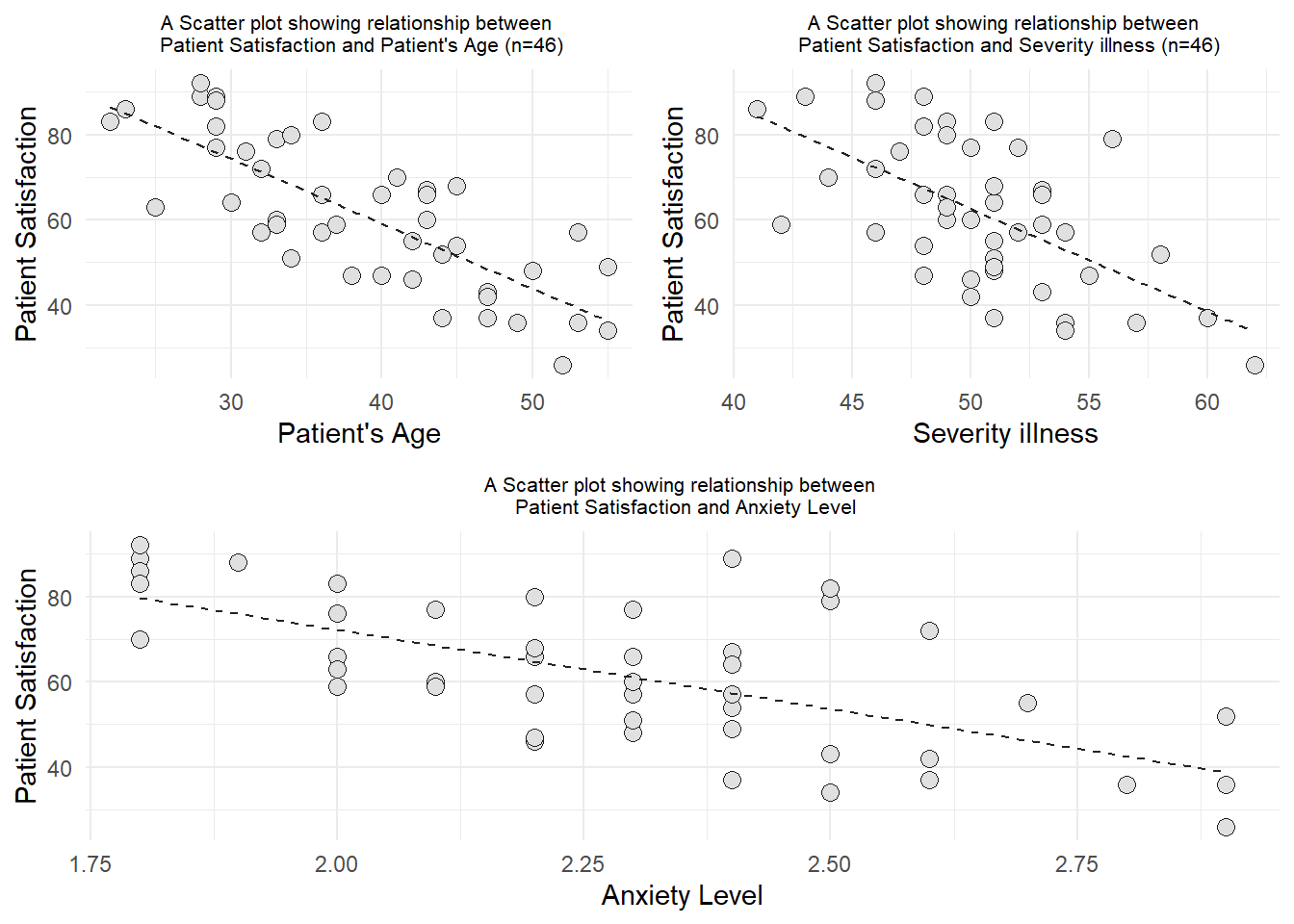
Based on the scatter diagrams, we can conclude that all of the variables (Age, Severity illness, and Anxiety level) have negatively linear correlation with Patient’s satisfaction.
Step 2: Univariable Analysis (Simple Linear Regression)
library(gtsummary)
data1 %>%
  select(everything()) %>%
  tbl_uvregression(
    method = glm,
    y=Y,
    hide_n= TRUE,
    pvalue_fun = ~style_pvalue(.x, digits = 3),
    # add_estimate_to_reference_rows = T,
    # statistic = all_continuous() ~ "{mean} ({sd})"
  ) %>%
  modify_column_unhide(columns = c(statistic, std.error)) %>%
  bold_p() %>%
  bold_labels() %>%
  add_global_p() %>%
  add_n(location = "level") %>%
  modify_caption("Table 3. Association of Patients Satisfaction and Combination of Factors (Age, illness, and Anxiety) (n=46)") %>%
  modify_header(label = "**Contributed Factors**") %>%
  modify_footnote(
ci = "CI = 95% Confidence Interval for Simple Linear Regression", abbreviation = TRUE) | Contributed Factors | N | Beta | SE1 | Statistic | 95% CI1 | p-value |
|---|---|---|---|---|---|---|
| Patient's Age (years) | 46 | -1.5 | 0.180 | -8.45 | -1.9, -1.2 | <0.001 |
| Severity illness (Index) | 46 | -2.4 | 0.481 | -5.01 | -3.4, -1.5 | <0.001 |
| Anxiety Level (index) | 46 | -37 | 6.64 | -5.59 | -50, -24 | <0.001 |
| 1 SE = Standard Error, CI = 95% Confidence Interval for Simple Linear Regression | ||||||
TIn Table 3, all variables exhibited a statistically significant relationship with patient satisfaction at the univariable level, as evidenced by the results of simple linear regression analyses. The association between patient satisfaction and age was found to be significant, with a p-value of less than 0.05 [t-statistic (df): -8.45 (44): p-value < 0.001]. Moreover, the negative beta coefficient (-1.5) suggests a negative relationship between these two variables. Additionally, 61.90% of the total variation in patient satisfaction was explained by patient’s age.
Similarly, a significant linear relationship was observed between patient satisfaction and severity of illness, with a p-value below 0.05 [t-statistic (df): -5.01 (44): p-value < 0.001]. The negative beta coefficient (-2.4) indicates a negative linear relationship, and the R-square value revealed that 36.35% of the total variation in patient satisfaction was explained by severity of illness.
In the case of patient satisfaction and anxiety level, a significant relationship was identified, supported by a p-value less than 0.05 [t-statistic (df): -5.59 (44); p-value < 0.001]. The considerable negative beta coefficient (-37.11) highlights a strong negative relationship between satisfaction and anxiety level. The R-square value further indicated that 41.55% of the total variation in patient satisfaction could be explained by anxiety level.
Checking the model assumptions for univariable analysis
- Patient Satisfaction and Patient’s Age
#Satisfaction and Age
SA <- lm(data1$Y~data1$x1)
#Linearity and Equality of variances
library(ggplot2)
#extracting the data from model
resid1 <- data.frame(cbind(residual = SA$residuals, predicted =SA$fitted.values))
#Scatter diagram
ggplot(resid1, aes(x=predicted, y=residual)) +
     geom_point(pch=21, size = 3.5, bg="grey88", col="grey56") +
     stat_ellipse(lty=2, color = "red") +
     theme_minimal() +
     ggtitle("Predicted vs Residual for linearity and equality of variances")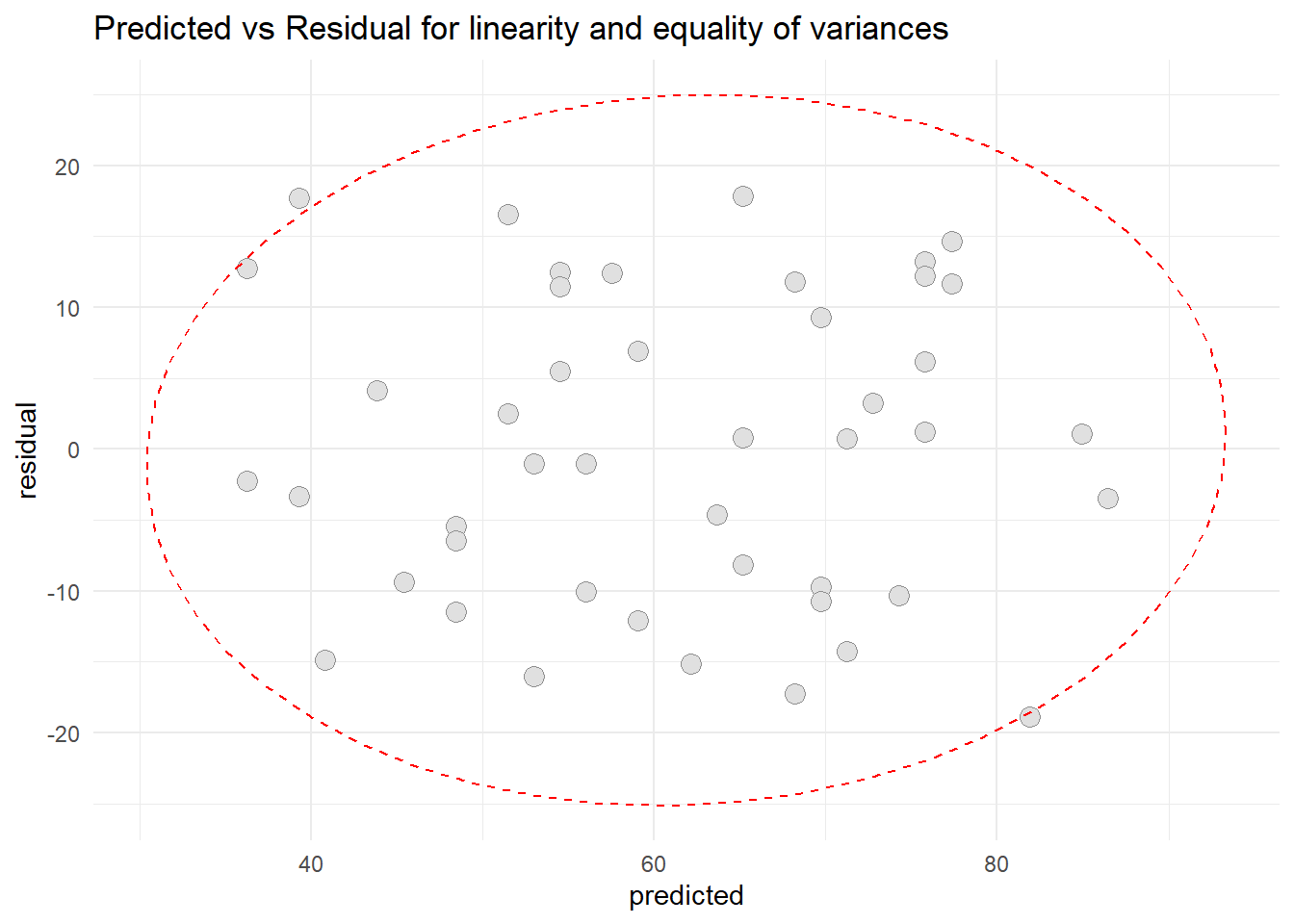
Based on scatter diagram of predicted vs residual, we can conclude that the linearity assumption and equality assumption were met.
#normality of the residuals
shapiro.test(resid1$residual)
    Shapiro-Wilk normality test

data:  resid1$residual
W = 0.95459, p-value = 0.0706
Based on the Shapiro Wilk test of normality, we can conclude that the distribution of the model residual is normally distributed since the p-value was more than 0.05 [W-Statistic: 0.9546; p-value: 0.0706].
- Patient satisfaction and Severity illness
#Satisfaction and Severity illness
SS <- lm(data1$Y~data1$x2)
#Linearity and Equality of variances
library(ggplot2)
#extracting the data from model
resid2 <- data.frame(cbind(residual = SS$residuals, predicted =SS$fitted.values))
#Scatter diagram
ggplot(resid2, aes(x=predicted, y=residual)) +
     geom_point(pch=21, size = 3.5, bg="grey88", col="grey56") +
     stat_ellipse(lty=2, color = "red") +
     theme_minimal() +
     ggtitle("Predicted vs Residual for linearity and equality of variances")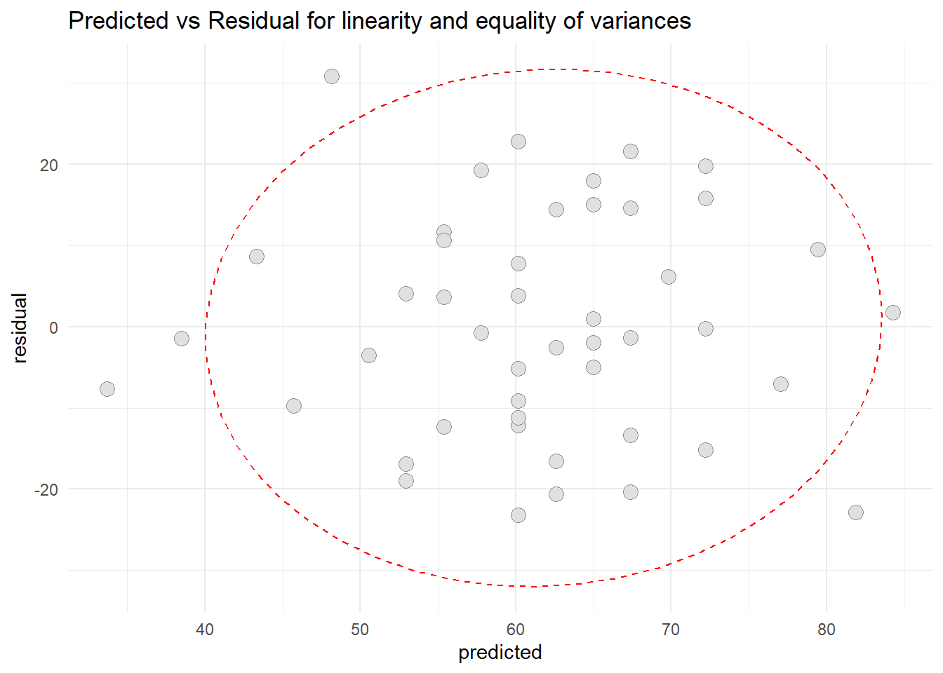
Based on scatter diagram of predicted vs residual for patient satisfaction and severity illness, we can conclude that the linearity assumption and equality assumption were met.
#normality of the residuals
shapiro.test(resid2$residual)
    Shapiro-Wilk normality test

data:  resid2$residual
W = 0.97706, p-value = 0.4911
Based on the Shapiro Wilk test of normality for patient satisfaction and severity illness, we can conclude that the distribution of the model residual is normally distributed since the p-value was more than 0.05 [W-Statistic: 0.97706; p-value: 0.4911].
- Patient satisfaction and Anxiety levels
#Satisfaction and Severity illness
SA2 <- lm(data1$Y~data1$x3)
#Linearity and Equality of variances
library(ggplot2)
#extracting the data from model
resid3 <- data.frame(cbind(residual = SA2$residuals, predicted =SA2$fitted.values))
#Scatter diagram
ggplot(resid3, aes(x=predicted, y=residual)) +
     geom_point(pch=21, size = 3.5, bg="grey88", col="grey56") +
     stat_ellipse(lty=2, color = "red") +
     theme_minimal() +
     ggtitle("Predicted vs Residual for linearity and equality of variances")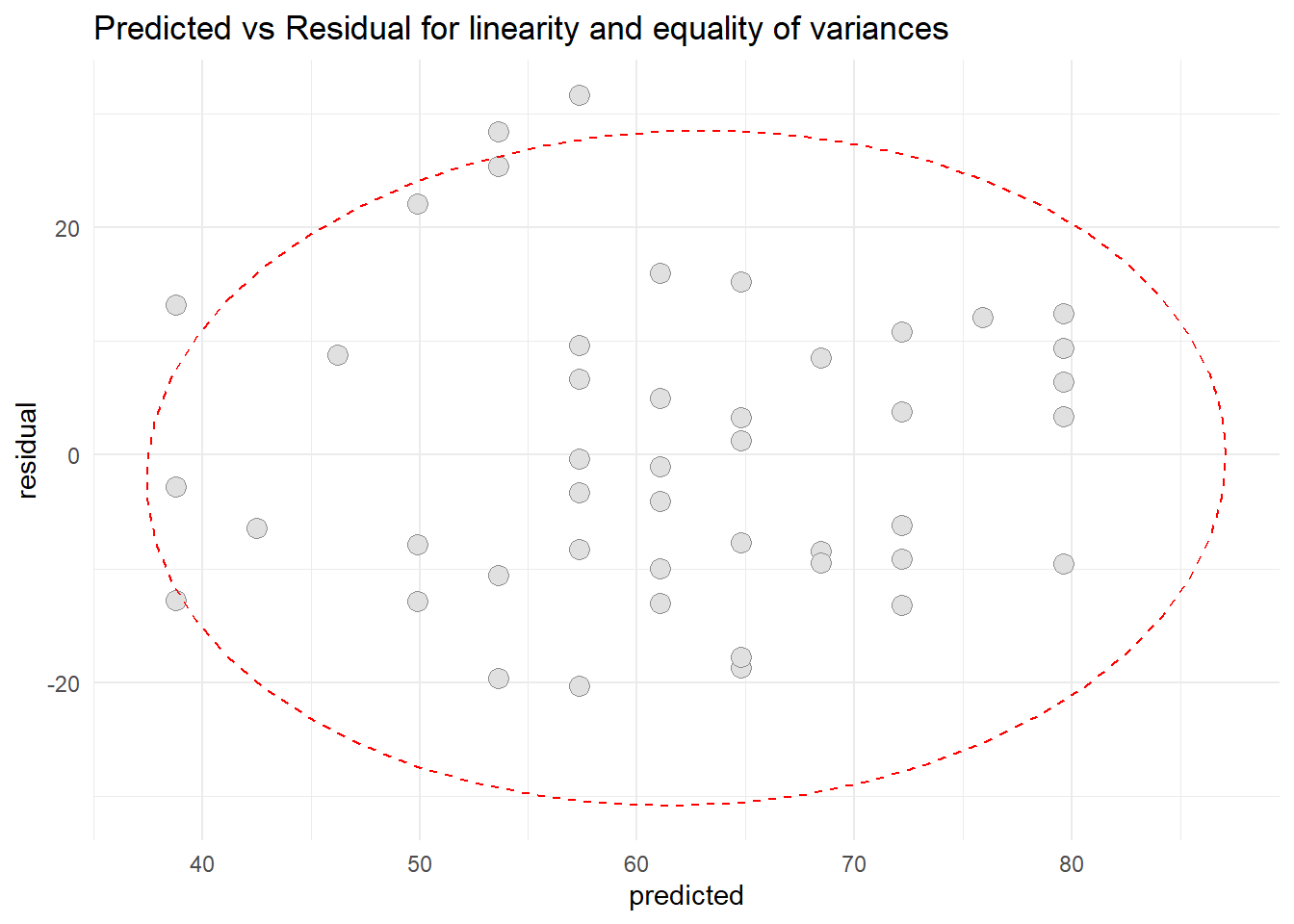
Based on scatter diagram of predicted vs residual for patient satisfaction and Anxiety level, we can conclude that the linearity assumption and equality assumption were met.
#normality of the residuals
shapiro.test(resid3$residual)
    Shapiro-Wilk normality test

data:  resid3$residual
W = 0.96017, p-value = 0.1164
Based on the Shapiro Wilk test of normality for patient satisfaction and Anxiety level, we can conclude that the distribution of the model residual is normally distributed since the p-value was more than 0.05 [W-Statistic: 0.97706; p-value: 0.4911].
Step 3: Variable Selection
The selection is done by using automatic procedure, where in R, there are forward, backward, and stepwise procedure. We can choose any of it, but some statisticians prefer to do all methods and review the results. But based on my experience, the best procedure is forward procedure because in forward procedure, most of the time it will comply the principle of variable selection.
The principle of variable selection:
1) Principle of fit of the model (means the higher number of variable, the model fitness getting better and better - but this may not be a preferred principle).
2) Principle of parsimony (means the model with least number of variable, but those variable are significant) - this is an important principle!.
3) Biologically plausibility (means that which variable are proven significant by literature) - we may need to use force enter if the tested variable is not significant.
When the variable selection procedure was performed, at this stage have preliminary main effect model.
Variable Selection procedure
First, we need to create empty model and full model. Empty model means only dependent variable is in the model. The Full model means all the independent variables are included into the model.
Empty Model
#Empty Model
EM <- lm(Y~1 , data=data1)
summary(EM)
Call:
lm(formula = Y ~ 1, data = data1)

Residuals:
    Min      1Q  Median      3Q     Max
-35.565 -13.315  -1.565  15.185  30.435

Coefficients:
            Estimate Std. Error t value Pr(>|t|)
(Intercept)   61.565      2.541   24.23   <2e-16 ***
---
Signif. codes:  0 '***' 0.001 '**' 0.01 '*' 0.05 '.' 0.1 ' ' 1

Residual standard error: 17.24 on 45 degrees of freedomformula(EM)Y ~ 1Based on this, there were no independent variable included in the model
Full Model
#Full Model
FM <- lm(Y ~ . , data=data1)
summary(FM)
Call:
lm(formula = Y ~ ., data = data1)

Residuals:
     Min       1Q   Median       3Q      Max
-18.3524  -6.4230   0.5196   8.3715  17.1601

Coefficients:
            Estimate Std. Error t value Pr(>|t|)
(Intercept) 158.4913    18.1259   8.744 5.26e-11 ***
x1           -1.1416     0.2148  -5.315 3.81e-06 ***
x2           -0.4420     0.4920  -0.898   0.3741
x3          -13.4702     7.0997  -1.897   0.0647 .
---
Signif. codes:  0 '***' 0.001 '**' 0.01 '*' 0.05 '.' 0.1 ' ' 1

Residual standard error: 10.06 on 42 degrees of freedom
Multiple R-squared:  0.6822,    Adjusted R-squared:  0.6595
F-statistic: 30.05 on 3 and 42 DF, p-value: 1.542e-10formula(FM)Y ~ x1 + x2 + x3Based on Full Model, we can see that all the independent variables were included into the model. We can noticed that the severity illness and Anxiety level were not significant when we include all the variables at once.
Forward Selection
In forward selection, the first variable selected for an entry into the constructed model is the one with the largest correlation with the dependent variable. Once the variable has been selected, it is evaluated on the based on certain criteria. The most common one are Mallow’s Cp or Akaike’s information criteria. If the first selected variables meets the criterion for inclusion, then the forward selection continues (the statistics for the variables not in the equation are used to select the next one). The procedure stops, when no other variables are left that meet the entry criterion.
#Forward Selection Procedure
forward1 <- step(EM,
                 direction = "forward",
                 scope = formula(FM))
Start: AIC=262.92
Y ~ 1
Df Sum of Sq RSS AIC
+ x1 1 8275.4 5093.9 220.53
+ x3 1 5554.9 7814.4 240.21
+ x2 1 4860.3 8509.0 244.13
<none> 13369.3 262.92
Step: AIC=220.53
Y ~ x1
Df Sum of Sq RSS AIC
+ x3 1 763.42 4330.5 215.06
+ x2 1 480.92 4613.0 217.97
<none> 5093.9 220.53
Step: AIC=215.06
Y ~ x1 + x3
Df Sum of Sq RSS AIC
<none> 4330.5 215.06
+ x2 1 81.659 4248.8 216.19summary(forward1)
Call:
lm(formula = Y ~ x1 + x3, data = data1)

Residuals:
     Min       1Q   Median       3Q      Max
-19.4453  -7.3285   0.6733   8.5126  18.0534

Coefficients:
            Estimate Std. Error t value Pr(>|t|)
(Intercept) 145.9412    11.5251  12.663 4.21e-16 ***
x1           -1.2005     0.2041  -5.882 5.43e-07 ***
x3          -16.7421     6.0808  -2.753  0.00861 **
---
Signif. codes:  0 '***' 0.001 '**' 0.01 '*' 0.05 '.' 0.1 ' ' 1

Residual standard error: 10.04 on 43 degrees of freedom
Multiple R-squared:  0.6761,    Adjusted R-squared:  0.661
F-statistic: 44.88 on 2 and 43 DF,  p-value: 2.98e-11
Based on the forward procedure, we can see that only variable patient’s age and anxiety level were included into the model. The severity illness was excluded from the model.
Backward Elimination
Backward elimination starts with all the variables in the equation and then it sequentially removes them. It is the simplest of all variable selection procedures and can be easily implemented without special software. In situation where there is a complex hierarchy, backward elimination can be run manually while taking account of what variables are eligible for removal. It start with all candidate variables in the model, then remove the variable with the largest p-value, that is, the variable that is the least statistically significant. The new (p-1)-variable model is t, and the variable with the largest p-value is removed. Continue until a stopping rule is reached. For instance, we may stop when all remaining variables have a significant p-value defined by some significance threshold.
In order to be able to perform backward elimination, we need to be in a situation where we have more observations than variables because we can do least squares regression when n (sample size) is greater than p (variables). If p is greater than n, we cannot fit a least squares model.
#Backward Elimination Procedure
backward <- step(FM,
                 direction = "backward")
Start: AIC=216.18
Y ~ x1 + x2 + x3
Df Sum of Sq RSS AIC
- x2 1 81.66 4330.5 215.06
<none> 4248.8 216.19
- x3 1 364.16 4613.0 217.97
- x1 1 2857.55 7106.4 237.84
Step: AIC=215.06
Y ~ x1 + x3
Df Sum of Sq RSS AIC
<none> 4330.5 215.06
- x3 1 763.4 5093.9 220.53
- x1 1 3483.9 7814.4 240.21summary(backward)
Call:
lm(formula = Y ~ x1 + x3, data = data1)

Residuals:
     Min       1Q   Median       3Q      Max
-19.4453  -7.3285   0.6733   8.5126  18.0534

Coefficients:
            Estimate Std. Error t value Pr(>|t|)
(Intercept) 145.9412    11.5251  12.663 4.21e-16 ***
x1           -1.2005     0.2041  -5.882 5.43e-07 ***
x3          -16.7421     6.0808  -2.753  0.00861 **
---
Signif. codes:  0 '***' 0.001 '**' 0.01 '*' 0.05 '.' 0.1 ' ' 1

Residual standard error: 10.04 on 43 degrees of freedom
Multiple R-squared:  0.6761,    Adjusted R-squared:  0.661
F-statistic: 44.88 on 2 and 43 DF,  p-value: 2.98e-11
Based on the backward procedure, we can see that only variable patient’s age and anxiety level were included into the model. The severity illness was excluded from the model. This result are same with the result produced from forward selection procedure.
Stepwise Selection
Stepwise selection is a procedure for variable selection in which all variables in a block are entered in a single step. At each step, the independent variable not in the equation that has the smallest probability of F is entered, if that probability is sufficiently small. Variables already in the regression equation are removed if their probability of F becomes sufficiently large. The method terminates when no more variables are eligible for inclusion or removal.
#Stepwise Selection Procedure
stepwise <- step(FM,
                 direction= "both")
Start: AIC=216.18
Y ~ x1 + x2 + x3
Df Sum of Sq RSS AIC
- x2 1 81.66 4330.5 215.06
<none> 4248.8 216.19
- x3 1 364.16 4613.0 217.97
- x1 1 2857.55 7106.4 237.84
Step: AIC=215.06
Y ~ x1 + x3
Df Sum of Sq RSS AIC
<none> 4330.5 215.06
+ x2 1 81.7 4248.8 216.19
- x3 1 763.4 5093.9 220.53
- x1 1 3483.9 7814.4 240.21summary(stepwise)
Call:
lm(formula = Y ~ x1 + x3, data = data1)

Residuals:
     Min       1Q   Median       3Q      Max
-19.4453  -7.3285   0.6733   8.5126  18.0534

Coefficients:
            Estimate Std. Error t value Pr(>|t|)
(Intercept) 145.9412    11.5251  12.663 4.21e-16 ***
x1           -1.2005     0.2041  -5.882 5.43e-07 ***
x3          -16.7421     6.0808  -2.753  0.00861 **
---
Signif. codes:  0 '***' 0.001 '**' 0.01 '*' 0.05 '.' 0.1 ' ' 1

Residual standard error: 10.04 on 43 degrees of freedom
Multiple R-squared:  0.6761,    Adjusted R-squared:  0.661
F-statistic: 44.88 on 2 and 43 DF,  p-value: 2.98e-11
Based on the stepwise procedure, we can see that only variable patient’s age and anxiety level were included into the model. The severity illness was excluded from the model. This result are same with the result produced from forward selection and backward elimination.
Since only Patient’s age and Anxiety level were included into the model for all the procedures. We now can establish our first model called as preliminary main effect model.
#Preliminary Main Effect Model
PMEM <- lm(Y~x1+x3, data=data1)
summary(PMEM)
Call:
lm(formula = Y ~ x1 + x3, data = data1)

Residuals:
     Min       1Q   Median       3Q      Max
-19.4453  -7.3285   0.6733   8.5126  18.0534

Coefficients:
            Estimate Std. Error t value Pr(>|t|)
(Intercept) 145.9412    11.5251  12.663 4.21e-16 ***
x1           -1.2005     0.2041  -5.882 5.43e-07 ***
x3          -16.7421     6.0808  -2.753  0.00861 **
---
Signif. codes:  0 '***' 0.001 '**' 0.01 '*' 0.05 '.' 0.1 ' ' 1

Residual standard error: 10.04 on 43 degrees of freedom
Multiple R-squared:  0.6761,    Adjusted R-squared:  0.661
F-statistic: 44.88 on 2 and 43 DF,  p-value: 2.98e-11
In this preliminary main effect model, the equation of the model is:
\[ patient Satisfaction = 145.94 - 1.20*Age(years) - 16.74*Anxiety level \]
Step 4: Checking Interaction
Interaction term needs to be computed. An interaction term is added to the model as an independent variable and to be check only one term at one time. If an interaction term is statistically significant, then the model should be main effect terms with the significant interaction term. This interaction term should be biologically meaningful.
#checking interaction term for Age and Anxiety

#Creating the interaction variable
data1$x1x3 <- data1$x1*data1$x3

InteractionAgeAnxiety <- lm(data1$Y~data1$x1+data1$x3+data1$x1x3)
summary(InteractionAgeAnxiety)
Call:
lm(formula = data1$Y ~ data1$x1 + data1$x3 + data1$x1x3)

Residuals:
    Min      1Q  Median      3Q     Max
-17.763  -7.873   1.517   9.306  16.439

Coefficients:
            Estimate Std. Error t value Pr(>|t|)
(Intercept)  89.9404    52.5535   1.711   0.0944 .
data1$x1      0.2598     1.3526   0.192   0.8486
data1$x3      8.0672    23.5140   0.343   0.7333
data1$x1x3   -0.6361     0.5825  -1.092   0.2810
---
Signif. codes:  0 '***' 0.001 '**' 0.01 '*' 0.05 '.' 0.1 ' ' 1

Residual standard error: 10.01 on 42 degrees of freedom
Multiple R-squared:  0.685, Adjusted R-squared:  0.6625
F-statistic: 30.45 on 3 and 42 DF,  p-value: 1.28e-10
For testing the interaction term age and anxiety, we can see that the interaction term is not significant in the model. Furthermore, there are no further interaction term to be tested. Thus, the model should only consist main effect variables.
Step 5: Checking Multicollinearity
Collinearity means there is an existence of correlation or relationship between independent variables. We need to check whether independent variables in previous step are correlated or not. If so, then there is a high chance of getting inaccurate p-value and wide 95% confidence interval of regression coefficient (we need to remove that variable or use other regression method). There are 2 method to check the multicollinearity:
1) Variance Inflation Factor (VIF), if VIF is more than 10, then there is a multicollinearity among independent variables.
2) Tolerance (TOL), if TOL is less than 0.2 then there is a multicollinearity among independent variables.
#checking multicollinearity
library(mctest)
imcdiag(PMEM)
Call:
imcdiag(mod = PMEM)


All Individual Multicollinearity Diagnostics Result

      VIF    TOL      Wi  Fi Leamer    CVIF Klein   IND1 IND2
x1 1.4805 0.6755 21.1401 Inf 0.8219 -13.907     0 0.0154    1
x3 1.4805 0.6755 21.1401 Inf 0.8219 -13.907     0 0.0154    1

1 --> COLLINEARITY is detected by the test
0 --> COLLINEARITY is not detected by the test

* all coefficients have significant t-ratios

R-square of y on all x: 0.6761

* use method argument to check which regressors may be the reason of collinearity
===================================
From the result, the VIF value is less than 10 for both independent variables. For TOL, the values are higher than 0.2 for both independent variables. Hence, we can conclude that the multicollinearity does not exist. We then, can proceed with the next step to establish preliminary final model.
Establishing Preliminary Final Model
The preliminary final model is:
PFM <- lm(data1$Y~ data1$x1+data1$x3)
summary(PFM)
Call:
lm(formula = data1$Y ~ data1$x1 + data1$x3)

Residuals:
     Min       1Q   Median       3Q      Max
-19.4453  -7.3285   0.6733   8.5126  18.0534

Coefficients:
            Estimate Std. Error t value Pr(>|t|)
(Intercept) 145.9412    11.5251  12.663 4.21e-16 ***
data1$x1     -1.2005     0.2041  -5.882 5.43e-07 ***
data1$x3    -16.7421     6.0808  -2.753  0.00861 **
---
Signif. codes:  0 '***' 0.001 '**' 0.01 '*' 0.05 '.' 0.1 ' ' 1

Residual standard error: 10.04 on 43 degrees of freedom
Multiple R-squared:  0.6761,    Adjusted R-squared:  0.661
F-statistic: 44.88 on 2 and 43 DF, p-value: 2.98e-11confint(PFM) 2.5 % 97.5 %
(Intercept) 122.698664 169.1837924
data1$x1 -1.612089 -0.7888539
data1$x3 -29.005215 -4.4788883Step 6: Checking Assumptions of the Model (LINE-I)
There are 5 main assumptions to be checked before establishing the final model. The assumptions to be check are: Linearity (L), Independence (I), Normality of the response variable (N), Homoscedasticity (Equal Variance) (E), and Fit of Independent numerical variable (I).
The description of each assumptions are as follows:
| Assumption | Description | Tools |
|---|---|---|
| Linearity (L) | The relationship between Xs and Y is linear over the range of values studied. | Scatter plot between residuals and predicted values (XP-YR) |
| Independence (I) | Independent Sample. | Settled during design stage |
| Normality of the response variable (N) | The response variable (Y), has a normal distribution at each value of the exploratory variables (Xs). | 1) Histogram with overlaid normal curve of residuals. 2) Box and Whisker plot of residuals. |
| Homoscedasticity (Equal Variance) (E) | The distribution of Y has equal variances (or standard deviation) at each value of Xs, that is, standard deviations of Y is same no matter what the value of Xs. | Scatter plot between residuals and predicted values. (XP-YR). |
| Fit of independent numerical variable (I) | There is no peculiar relationship between independent numerical variables and outcome variable. Independent numerical variables have linear relationship with the outcome. | Scatter plot between residual and predicted values (XI-YR). |
- Checking Linearity and Homoscedasticity
For linearity, if there any unusual shape of concavity or convexity of fitted observation, the the assumption is not met. For equal variances, if there is a unusual shape of divergence or fan-shape of fitted observation, then the assumption is not met.
#Extracting the residual and predicted variables
resid4 <- data.frame(cbind(residual = PFM$residuals,
                           predicted =PFM$fitted.values))

#Scatter diagram between residuals and predicted values
library(ggplot2)
ggplot(resid4, aes(x=predicted, y=residual)) +
  geom_point(pch=21, size = 3.5, bg="grey88", col="grey56") +
  stat_ellipse(lty=2, color = "red") +
  theme_minimal() +
  ggtitle("Predicted vs Residual for linearity and equality of variances")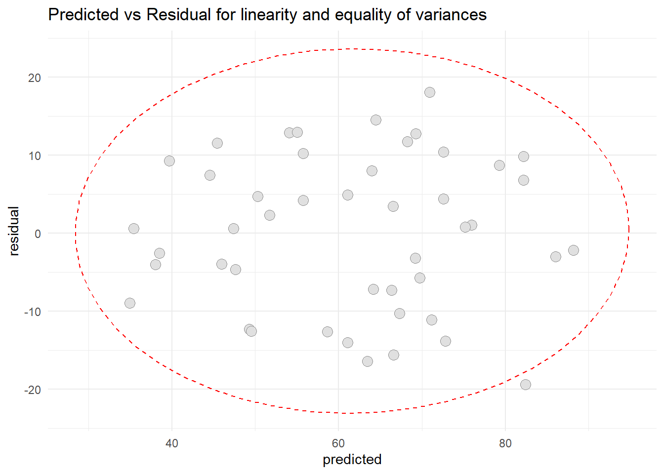
Based on the graph, we can conclude that the residual appears linear and randomly scattered. Thus the assumption of equality of variance is met and assumption of linearity also met.
- Checking Normality of the residuals.
#boxplot of the residuals
ggplot(resid4, aes(x=residual)) +
  geom_boxplot() +
  theme_minimal()+
  scale_y_continuous(limits=c(-1,1)) +
  labs(title = "A Boxplot plot showing distribution of the residual",
       x = "Residual") +
  theme(plot.title = element_text(hjust=0.5))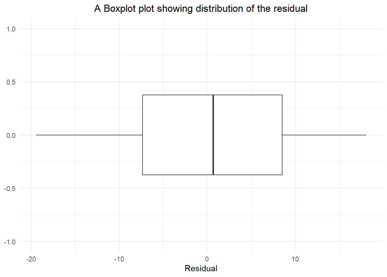
#shapiro wilk normality test
shapiro.test(resid4$residual)
    Shapiro-Wilk normality test

data:  resid4$residual
W = 0.96529, p-value = 0.1838
Based on the boxplot of the residual, we can conclude that the data is normally distributed. In addition, based on Shapiro Wilk test of normality, it shows that the p-value was more than 0.05 [W-Statistic: 0.96529; p-value: 0.1838]. Hence, the assumptions of normality of the residual is met.
- Linearity of the independent variables
library(ggplot2)
library(gridExtra)
#Scatter plot for Age and Residual
AR <- ggplot(resid4, aes(x=data1$x1, y=residual)) +
      geom_point(pch=21, size = 3.5, bg="grey88", col="grey56") +
      stat_ellipse(lty=2, color = "red") +
      theme_minimal() +
      labs( title = "Age vs Residual for Linearity of Independence variable",
            x = "Patient's Age",
            y = "Residual") +
  theme(plot.title = element_text(hjust=0.5))

#Scatter plot for Anxiety and Residual
AR2 <- ggplot(resid4, aes(x=data1$x3, y=residual)) +
      geom_point(pch=21, size = 3.5, bg="grey88", col="grey56") +
      stat_ellipse(lty=2, color = "red") +
      theme_minimal() +
      labs( title = "Age vs Residual for Linearity of Independence variable",
            x = "Anxiety Level",
            y = "Residual") +
  theme(plot.title = element_text(hjust=0.5))

grid.arrange(arrangeGrob(AR,AR2), nrow = 1)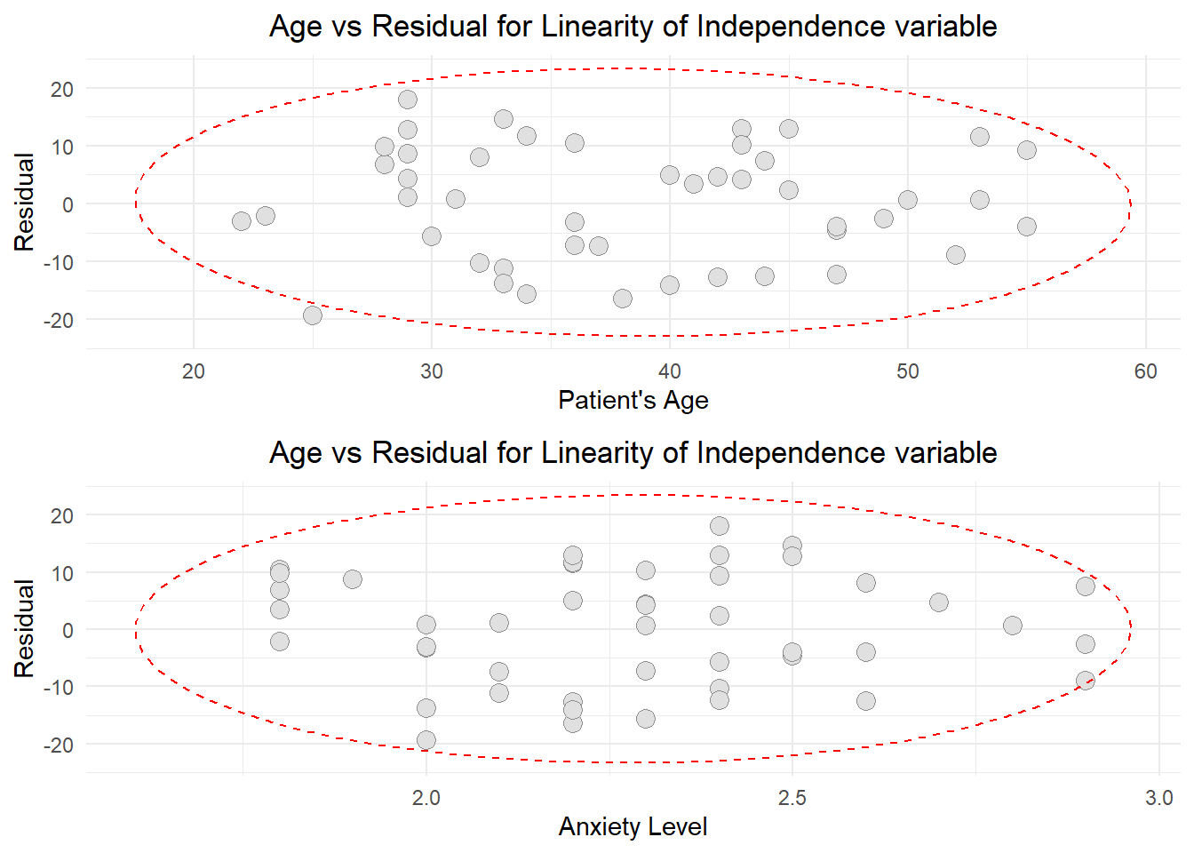
Based on the graphs, there are no unusual relationship between independent numerical variables and residuals. The forms of independent numerical variables (Patient’s age and Anxiety Level) are appropriate. They have linear relationship with the residuals. Thus the assumption of fit of independent numerical variables were met.
Step 7: Establishing Final Model
After thorough checking, we now can establish the final model to explain the patient satisfaction in the hospital. The final model are:
Final <- lm(data1$Y ~ data1$x1 + data1$x3)
summary(Final)
Call:
lm(formula = data1$Y ~ data1$x1 + data1$x3)

Residuals:
     Min       1Q   Median       3Q      Max
-19.4453  -7.3285   0.6733   8.5126  18.0534

Coefficients:
            Estimate Std. Error t value Pr(>|t|)
(Intercept) 145.9412    11.5251  12.663 4.21e-16 ***
data1$x1     -1.2005     0.2041  -5.882 5.43e-07 ***
data1$x3    -16.7421     6.0808  -2.753  0.00861 **
---
Signif. codes:  0 '***' 0.001 '**' 0.01 '*' 0.05 '.' 0.1 ' ' 1

Residual standard error: 10.04 on 43 degrees of freedom
Multiple R-squared:  0.6761,    Adjusted R-squared:  0.661
F-statistic: 44.88 on 2 and 43 DF, p-value: 2.98e-11confint(Final) 2.5 % 97.5 %
(Intercept) 122.698664 169.1837924
data1$x1 -1.612089 -0.7888539
data1$x3 -29.005215 -4.4788883To report the multiple linear regression, we need to pay attention on the relationship or the purpose of the analysis in text. Explain about the sample size, Regression coefficient, their 95% confidence interval and the actual p-value of each independent variable in the final model. Furthermore, we need to explain the coefficient of determination and confirm that the assumptions are fulfilled (in text and footnote of the table). Next, inform about the interactions and multicollinearity problem. Then report how any outlying data are treated (example: transformation of data if normality assumption is not met (in text)). Lastly, state the statistical package used in the analysis.
Step 8: Presentation of the Results
Suggested Interpretation:
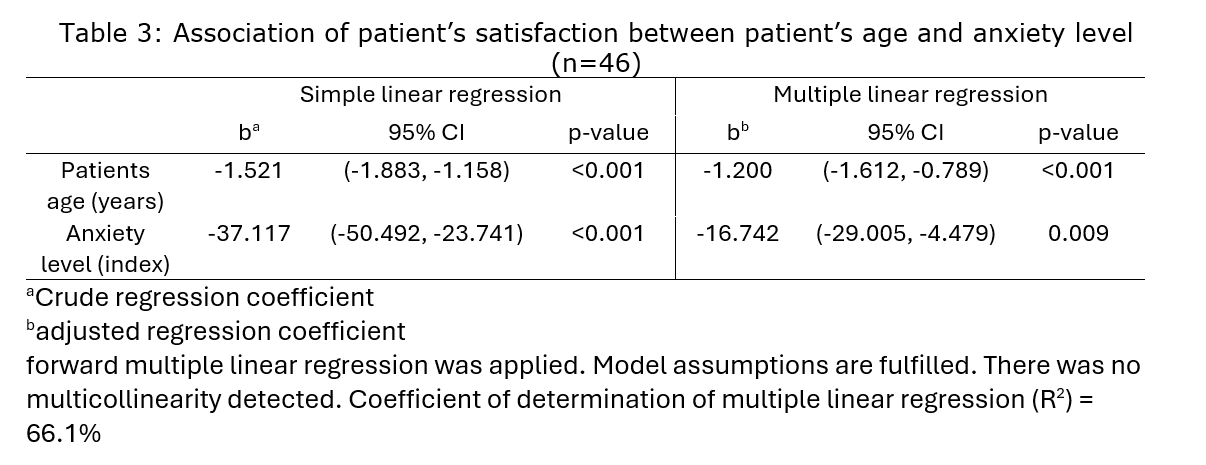
The multiple linear regression analysis aimed to explore the relationship between patient satisfaction (Y) and independent variables, patient’s age (x1) and anxiety level (x3). The analysis was conducted on a sample size of 46 patients. The study encompassed data from 46 patients, providing a robust foundation for the multiple linear regression analysis. In the final model, the regression coefficients for patient’s age (x1) and anxiety level (x3) were estimated at -1.2005 (95% CI [-1.6121, -0.7889]) and -16.7421 (95% CI [-29.0052, -4.4789]) respectively. These coefficients signify the expected change in patient satisfaction for a one-unit increase in the corresponding independent variable, holding other variables constant. The p-values associated with patient’s age (x1) and anxiety level (x3) were both statistically significant (p < 0.05), indicating a significant impact on patient satisfaction. The coefficient of determination (R-squared) was found to be 0.6761, suggesting that approximately 67.61% of the variance in patient satisfaction could be explained by the combined influence of patient’s age and anxiety level. The adjusted R-squared, accounting for the number of predictors, was 0.661. Assumption checks were meticulously conducted. Linearity, equality of variance, normality, and linearity of independent variables were assessed and confirmed. The residuals displayed a reasonable distribution.
Variable selection procedures (forward selection, backward selection, and stepwise) unanimously identified that severity of illness (noted as data1$x2) was not a significant predictor and was consequently excluded from the model. Interaction tests between patient’s age and anxiety level did not reveal any significant interaction effects. A multicollinearity test confirmed the absence of multicollinearity issues among the independent variables. The analysis was conducted using the lm function in R.
In summary, the multiple linear regression analysis highlights a substantial influence of patient’s age and anxiety level on patient satisfaction, with rigorous attention paid to assumptions, variable selection, interaction tests, and multicollinearity checks. The model exhibited a high explanatory power, capturing over two-thirds of the variance in patient satisfaction.
Exercise
1) Use pefr mlr.dta dataset from this link: https://sta334.s3.ap-southeast-1.amazonaws.com/data/pefr+mlr.dta. Perform multiple linear regression to find the relationship between PEFR and predictors (age, weight, and height). Check all the assumptions and procedures. Write an appropriate report for this analysis.
2) Conduct a multiple linear regression analysis with Sepal.length as the dependent variable and Sepal.width, petal.width, and petal.width as independent variable in the iris dataset. Test all the assumptions and interpret the results. Interpret the coefficients, R-squared, and adjusted R-squared values.
3) Conduct a multiple linear regression analysis with mpg as the dependent variable and hp, wt, and qsec as independent variables in the mtcars dataset. Test all the assumptions and interpret the results. Interpret the coefficients, R-squared and adjusted R-squared.
4) Find another dataset and perform both simple and multiple linear regression analyses. Check all assumptions and interpret the findings.
5) Choose a dataset and perform a multiple linear regression analysis with one dependent and at least 5 independent variables of your choice. Test all the assumptions and interpret the results.