library(nycflights13)
library(tidyverse)
library(dplyr)Introduction to dplyr
Introduction to dplyr package
Visualization is an important tool for insight generation, but it is rare that you get the data in exactly the right form you need. Often, you’ll need to create some new variables or summaries, or maybe you just want to rename the variables or reorder the observations in order to make the data a little easier to work with. You’ll learn how to do all that (and more!) in this note, which will teach you how to transform your data using the dplyr package and a new dataset on flights departing New York City in 2013.
Pre-requisite
In this note, we are going to focus on how to use the dplyr package, another core member of the tidyverse. We will illustrate the key ideas using data from the nycflights13 package and use ggplot2 to help us understand the data.
Take careful note of the conflicts message that’s printed when you load the tidyverse. It tells you that dplyr overwrites some functions in base R. If you want to use the base version of these functions after loading dplyr, you’ll need to use their full names: stats::filter() and stats::lag().
nycflights13
To explore the basic data manipulation verbs of dplyr, we’ll use nycflights13::flights. This data frame contains all 336,776 flights that departed from New York City in 2013. The data comes from the US Bureau of Transportation Statistics, and is documented in ?flights:
flights# A tibble: 336,776 × 19
year month day dep_time sched_dep_time dep_delay arr_time sched_arr_time
<int> <int> <int> <int> <int> <dbl> <int> <int>
1 2013 1 1 517 515 2 830 819
2 2013 1 1 533 529 4 850 830
3 2013 1 1 542 540 2 923 850
4 2013 1 1 544 545 -1 1004 1022
5 2013 1 1 554 600 -6 812 837
6 2013 1 1 554 558 -4 740 728
7 2013 1 1 555 600 -5 913 854
8 2013 1 1 557 600 -3 709 723
9 2013 1 1 557 600 -3 838 846
10 2013 1 1 558 600 -2 753 745
# ℹ 336,766 more rows
# ℹ 11 more variables: arr_delay <dbl>, carrier <chr>, flight <int>,
# tailnum <chr>, origin <chr>, dest <chr>, air_time <dbl>, distance <dbl>,
# hour <dbl>, minute <dbl>, time_hour <dttm>You might notice that this data frame prints a little differently from other data frames you might have used in the past: it only shows the first few rows and all the columns that fit on one screen. (To see the whole dataset, you can run View(flights), which will open the dataset in the RStudio viewer.) It prints differently because it’s a tibble. Tibbles are data frames, but slightly tweaked to work better in the tidyverse. For now, you don’t need to worry about the differences;
You might also have noticed the row of three- (or four-) letter abbreviations under the column names.
These describe the type of each variable:
• int stands for integers.
• dbl stands for doubles, or real numbers.
• chr stands for character vectors, or strings.
• dttm stands for date-times (a date + a time).
• lgl stands logical vectors that contain only TRUE or FALSE.
• fctr stands for factors, which R uses to represent categorical variable fixed possible values.
• date stands for dates.
dplyrBasics
In this notes you are going to learn the five key dplyr functions that allow you to solve the vast majority of your data-manipulation challenges:
• Pick observations by their values (filter()).
• Reorder the rows (arrange()).
• Pick variables by their names (select()).
• Create new variables with functions of existing variables (mutate()).
• Collapse many values down to a single summary (summarize()).
These can all be used in conjunction with group_by(), which changes the scope of each function from operating on the entire dataset to operating on it group-by-group. These six functions provide the verbs for a language of data manipulation. All verbs work similarly:
1. The first argument is a data frame.
2. The subsequent arguments describe what to do with the data frame, using the variable names (without quotes).
3. The result is a new data frame.
Together these properties make it easy to chain together multiple simple steps to achieve a complex result. Let’s dive in and see how these verbs work.
Filter row with filter()
filter() allows you to subset observations based on their values. The first argument is the name of the data frame. The second and subsequent arguments are the expressions that filter the data frame.
For example, we can select all flights on January 1st with:
filter(flights, month==1, day == 1)# A tibble: 842 × 19
year month day dep_time sched_dep_time dep_delay arr_time sched_arr_time
<int> <int> <int> <int> <int> <dbl> <int> <int>
1 2013 1 1 517 515 2 830 819
2 2013 1 1 533 529 4 850 830
3 2013 1 1 542 540 2 923 850
4 2013 1 1 544 545 -1 1004 1022
5 2013 1 1 554 600 -6 812 837
6 2013 1 1 554 558 -4 740 728
7 2013 1 1 555 600 -5 913 854
8 2013 1 1 557 600 -3 709 723
9 2013 1 1 557 600 -3 838 846
10 2013 1 1 558 600 -2 753 745
# ℹ 832 more rows
# ℹ 11 more variables: arr_delay <dbl>, carrier <chr>, flight <int>,
# tailnum <chr>, origin <chr>, dest <chr>, air_time <dbl>, distance <dbl>,
# hour <dbl>, minute <dbl>, time_hour <dttm>When you run that line of code, dplyr executes the filtering operation and returns a new data frame. dplyr functions never modify their inputs, so if you want to save the result, you’ll need to use the assignment operator, <-:
jan1st <- filter(flights, month==1, day == 1)R either prints out the results or saves them to a variable. If you want to do both, you can wrap the assignment in parentheses:
(dec25 <- filter(flights, month==12, day==25))# A tibble: 719 × 19
year month day dep_time sched_dep_time dep_delay arr_time sched_arr_time
<int> <int> <int> <int> <int> <dbl> <int> <int>
1 2013 12 25 456 500 -4 649 651
2 2013 12 25 524 515 9 805 814
3 2013 12 25 542 540 2 832 850
4 2013 12 25 546 550 -4 1022 1027
5 2013 12 25 556 600 -4 730 745
6 2013 12 25 557 600 -3 743 752
7 2013 12 25 557 600 -3 818 831
8 2013 12 25 559 600 -1 855 856
9 2013 12 25 559 600 -1 849 855
10 2013 12 25 600 600 0 850 846
# ℹ 709 more rows
# ℹ 11 more variables: arr_delay <dbl>, carrier <chr>, flight <int>,
# tailnum <chr>, origin <chr>, dest <chr>, air_time <dbl>, distance <dbl>,
# hour <dbl>, minute <dbl>, time_hour <dttm>Comparisons
To use filtering effectively, you have to know how to select the observations that you want using the comparison operators. R provides the standard suite: >, >=, <, <=, != (not equal), and == (equal).
When you’re starting out with R, the easiest mistake to make is to use = instead of == when testing for equality. When this happens, you’ll get an informative error:
filter(flights, month =1)
#> Error: filter() takes unnamed arguments. Do you need `==`?
Sometimes you can simplify complicated subsetting by remembering De Morgan’s law:
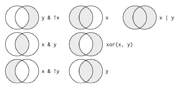
• !(x & y) is the same as !x | !y
• !(x | y) us the same as !x & !y
For example, if you wanted to find flights that weren’t delayed (on arrival or departure) by more than two hours, you could use either of the following two filter:
filter(flights, !(arr_delay > 120 | dep_delay >120))

filter(flights, arr_delay <= 120, dep_delay <=120)
Logical Operators
Multiple arguments to filter() are combined with “and”: every expression must be true in order for a row to be included in the output. For other types of combinations, you’ll need to use Boolean operators yourself: & is “and,” | is “or,” and ! is “not.” The following figure shows the complete set of Boolean operations.
The following code finds all flights that departed in November or December:
filter(flights, month==11, month ==12)# A tibble: 0 × 19
# ℹ 19 variables: year <int>, month <int>, day <int>, dep_time <int>,
# sched_dep_time <int>, dep_delay <dbl>, arr_time <int>,
# sched_arr_time <int>, arr_delay <dbl>, carrier <chr>, flight <int>,
# tailnum <chr>, origin <chr>, dest <chr>, air_time <dbl>, distance <dbl>,
# hour <dbl>, minute <dbl>, time_hour <dttm>The order of operations doesn’t work like English. You can’t write filter(flights, month == 11 | 12), which you might literally translate into “finds all flights that departed in November or December.”
A useful shorthand for this problem is x %in% y. This will select every row where x is one of the values in y. We could use it to rewrite the preceding code:
nov_dec <- filter(flights, month %in% c(11,12))Sometimes you can simplify complicated subsetting by remembering De Morgan’s law: !(x & y) is the same as !x | !y, and !(x | y) is the same as !x & !y. For example, if you wanted to find flights that weren’t delayed (on arrival or departure) by more than two hours, you could use either of the following two filters:
filter(flights, !(arr_delay > 120 | dep_delay > 120))# A tibble: 316,050 × 19
year month day dep_time sched_dep_time dep_delay arr_time sched_arr_time
<int> <int> <int> <int> <int> <dbl> <int> <int>
1 2013 1 1 517 515 2 830 819
2 2013 1 1 533 529 4 850 830
3 2013 1 1 542 540 2 923 850
4 2013 1 1 544 545 -1 1004 1022
5 2013 1 1 554 600 -6 812 837
6 2013 1 1 554 558 -4 740 728
7 2013 1 1 555 600 -5 913 854
8 2013 1 1 557 600 -3 709 723
9 2013 1 1 557 600 -3 838 846
10 2013 1 1 558 600 -2 753 745
# ℹ 316,040 more rows
# ℹ 11 more variables: arr_delay <dbl>, carrier <chr>, flight <int>,
# tailnum <chr>, origin <chr>, dest <chr>, air_time <dbl>, distance <dbl>,
# hour <dbl>, minute <dbl>, time_hour <dttm>filter(flights, arr_delay <= 120, dep_delay <= 120)# A tibble: 316,050 × 19
year month day dep_time sched_dep_time dep_delay arr_time sched_arr_time
<int> <int> <int> <int> <int> <dbl> <int> <int>
1 2013 1 1 517 515 2 830 819
2 2013 1 1 533 529 4 850 830
3 2013 1 1 542 540 2 923 850
4 2013 1 1 544 545 -1 1004 1022
5 2013 1 1 554 600 -6 812 837
6 2013 1 1 554 558 -4 740 728
7 2013 1 1 555 600 -5 913 854
8 2013 1 1 557 600 -3 709 723
9 2013 1 1 557 600 -3 838 846
10 2013 1 1 558 600 -2 753 745
# ℹ 316,040 more rows
# ℹ 11 more variables: arr_delay <dbl>, carrier <chr>, flight <int>,
# tailnum <chr>, origin <chr>, dest <chr>, air_time <dbl>, distance <dbl>,
# hour <dbl>, minute <dbl>, time_hour <dttm>Example 1
Filter flights that departed from JFK or LGA airports on a 15th and 20th of each months
filter(flights, (origin == "JFK" | origin == "LGA") &
         (day %in% c(15, 20)))
# A tibble: 14,355 × 19
year month day dep_time sched_dep_time dep_delay arr_time sched_arr_time
<int> <int> <int> <int> <int> <dbl> <int> <int>
1 2013 1 15 533 530 3 839 831
2 2013 1 15 534 540 -6 829 850
3 2013 1 15 535 540 -5 1014 1017
4 2013 1 15 543 600 -17 710 715
5 2013 1 15 552 600 -8 934 910
6 2013 1 15 552 600 -8 658 658
7 2013 1 15 554 600 -6 841 815
8 2013 1 15 554 600 -6 850 904
9 2013 1 15 554 600 -6 914 837
10 2013 1 15 554 600 -6 751 759
# ℹ 14,345 more rows
# ℹ 11 more variables: arr_delay <dbl>, carrier <chr>, flight <int>,
# tailnum <chr>, origin <chr>, dest <chr>, air_time <dbl>, distance <dbl>,
# hour <dbl>, minute <dbl>, time_hour <dttm>Example 2
Filter flights that departed on either the 1st or the 15th of any month and were operated by either “United” or “Delta” airlines.
filter(flights, (day %in% c(1,15)) & (carrier %in% c("UA", "DL")))# A tibble: 7,065 × 19
year month day dep_time sched_dep_time dep_delay arr_time sched_arr_time
<int> <int> <int> <int> <int> <dbl> <int> <int>
1 2013 1 1 517 515 2 830 819
2 2013 1 1 533 529 4 850 830
3 2013 1 1 554 600 -6 812 837
4 2013 1 1 554 558 -4 740 728
5 2013 1 1 558 600 -2 924 917
6 2013 1 1 558 600 -2 923 937
7 2013 1 1 559 600 -1 854 902
8 2013 1 1 602 610 -8 812 820
9 2013 1 1 606 610 -4 837 845
10 2013 1 1 607 607 0 858 915
# ℹ 7,055 more rows
# ℹ 11 more variables: arr_delay <dbl>, carrier <chr>, flight <int>,
# tailnum <chr>, origin <chr>, dest <chr>, air_time <dbl>, distance <dbl>,
# hour <dbl>, minute <dbl>, time_hour <dttm>Example 3
Filter flights that did not depart between 6 AM and 12 PM (noon).
filter(flights, !(hour >= 6 & hour <= 12))# A tibble: 189,528 × 19
year month day dep_time sched_dep_time dep_delay arr_time sched_arr_time
<int> <int> <int> <int> <int> <dbl> <int> <int>
1 2013 1 1 517 515 2 830 819
2 2013 1 1 533 529 4 850 830
3 2013 1 1 542 540 2 923 850
4 2013 1 1 544 545 -1 1004 1022
5 2013 1 1 554 558 -4 740 728
6 2013 1 1 559 559 0 702 706
7 2013 1 1 848 1835 853 1001 1950
8 2013 1 1 1255 1300 -5 1541 1537
9 2013 1 1 1255 1300 -5 1401 1409
10 2013 1 1 1257 1300 -3 1454 1450
# ℹ 189,518 more rows
# ℹ 11 more variables: arr_delay <dbl>, carrier <chr>, flight <int>,
# tailnum <chr>, origin <chr>, dest <chr>, air_time <dbl>, distance <dbl>,
# hour <dbl>, minute <dbl>, time_hour <dttm>Example 4
Filter flights that originated from JFK or LGA airports, but not in the month of February.
filter(flights, (origin == "JFK" | origin == "LGA") & month != 2)# A tibble: 200,097 × 19
year month day dep_time sched_dep_time dep_delay arr_time sched_arr_time
<int> <int> <int> <int> <int> <dbl> <int> <int>
1 2013 1 1 533 529 4 850 830
2 2013 1 1 542 540 2 923 850
3 2013 1 1 544 545 -1 1004 1022
4 2013 1 1 554 600 -6 812 837
5 2013 1 1 557 600 -3 709 723
6 2013 1 1 557 600 -3 838 846
7 2013 1 1 558 600 -2 753 745
8 2013 1 1 558 600 -2 849 851
9 2013 1 1 558 600 -2 853 856
10 2013 1 1 558 600 -2 924 917
# ℹ 200,087 more rows
# ℹ 11 more variables: arr_delay <dbl>, carrier <chr>, flight <int>,
# tailnum <chr>, origin <chr>, dest <chr>, air_time <dbl>, distance <dbl>,
# hour <dbl>, minute <dbl>, time_hour <dttm>Example 5
Filter flights that departed either before 5 AM or after 10 PM, and were operated by “American” or “JetBlue” airlines.
filter(flights, (hour < 5 | hour > 22) & carrier %in% c("AA", "B6"))# A tibble: 1,039 × 19
year month day dep_time sched_dep_time dep_delay arr_time sched_arr_time
<int> <int> <int> <int> <int> <dbl> <int> <int>
1 2013 1 1 2353 2359 -6 425 445
2 2013 1 1 2353 2359 -6 418 442
3 2013 1 1 2356 2359 -3 425 437
4 2013 1 2 42 2359 43 518 442
5 2013 1 2 2351 2359 -8 427 445
6 2013 1 2 2354 2359 -5 413 437
7 2013 1 3 32 2359 33 504 442
8 2013 1 3 235 2359 156 700 437
9 2013 1 3 2349 2359 -10 434 445
10 2013 1 4 25 2359 26 505 442
# ℹ 1,029 more rows
# ℹ 11 more variables: arr_delay <dbl>, carrier <chr>, flight <int>,
# tailnum <chr>, origin <chr>, dest <chr>, air_time <dbl>, distance <dbl>,
# hour <dbl>, minute <dbl>, time_hour <dttm>Example 6
Using palmerpenguins library, Filter for Adélie penguins that were observed on either the Torgersen or Dream Island.
library(palmerpenguins)Warning: package 'palmerpenguins' was built under R version 4.2.3filter(penguins, species == "Adelie" & island %in% c("Torgersen", "Dream"))# A tibble: 108 × 8
species island bill_length_mm bill_depth_mm flipper_length_mm body_mass_g
<fct> <fct> <dbl> <dbl> <int> <int>
1 Adelie Torgersen 39.1 18.7 181 3750
2 Adelie Torgersen 39.5 17.4 186 3800
3 Adelie Torgersen 40.3 18 195 3250
4 Adelie Torgersen NA NA NA NA
5 Adelie Torgersen 36.7 19.3 193 3450
6 Adelie Torgersen 39.3 20.6 190 3650
7 Adelie Torgersen 38.9 17.8 181 3625
8 Adelie Torgersen 39.2 19.6 195 4675
9 Adelie Torgersen 34.1 18.1 193 3475
10 Adelie Torgersen 42 20.2 190 4250
# ℹ 98 more rows
# ℹ 2 more variables: sex <fct>, year <int>Example 7
Filter for male penguins that were not observed on Biscoe Island.
filter(penguins, sex == "male" & !island == "Biscoe")# A tibble: 85 × 8
species island bill_length_mm bill_depth_mm flipper_length_mm body_mass_g
<fct> <fct> <dbl> <dbl> <int> <int>
1 Adelie Torgersen 39.1 18.7 181 3750
2 Adelie Torgersen 39.3 20.6 190 3650
3 Adelie Torgersen 39.2 19.6 195 4675
4 Adelie Torgersen 38.6 21.2 191 3800
5 Adelie Torgersen 34.6 21.1 198 4400
6 Adelie Torgersen 42.5 20.7 197 4500
7 Adelie Torgersen 46 21.5 194 4200
8 Adelie Dream 37.2 18.1 178 3900
9 Adelie Dream 40.9 18.9 184 3900
10 Adelie Dream 39.2 21.1 196 4150
# ℹ 75 more rows
# ℹ 2 more variables: sex <fct>, year <int>Example 8
Filter for penguins observed in the year 2008, excluding those with bill lengths less than 40 mm.
filter(penguins, year == 2008 & !(bill_length_mm < 40))# A tibble: 83 × 8
species island bill_length_mm bill_depth_mm flipper_length_mm body_mass_g
<fct> <fct> <dbl> <dbl> <int> <int>
1 Adelie Biscoe 40.1 18.9 188 4300
2 Adelie Biscoe 42 19.5 200 4050
3 Adelie Biscoe 41.4 18.6 191 3700
4 Adelie Biscoe 40.6 18.8 193 3800
5 Adelie Biscoe 41.3 21.1 195 4400
6 Adelie Biscoe 41.1 18.2 192 4050
7 Adelie Biscoe 41.6 18 192 3950
8 Adelie Biscoe 41.1 19.1 188 4100
9 Adelie Torgersen 41.8 19.4 198 4450
10 Adelie Torgersen 45.8 18.9 197 4150
# ℹ 73 more rows
# ℹ 2 more variables: sex <fct>, year <int>Example 9
Filter for penguins with a body mass between 3500 and 4500 grams that were observed on either Dream or Biscoe Island.
filter(penguins, body_mass_g >= 3500 & body_mass_g <= 4500 & island %in% c("Dream", "Biscoe"))# A tibble: 125 × 8
species island bill_length_mm bill_depth_mm flipper_length_mm body_mass_g
<fct> <fct> <dbl> <dbl> <int> <int>
1 Adelie Biscoe 37.7 18.7 180 3600
2 Adelie Biscoe 35.9 19.2 189 3800
3 Adelie Biscoe 38.2 18.1 185 3950
4 Adelie Biscoe 38.8 17.2 180 3800
5 Adelie Biscoe 35.3 18.9 187 3800
6 Adelie Biscoe 40.6 18.6 183 3550
7 Adelie Biscoe 40.5 18.9 180 3950
8 Adelie Dream 37.2 18.1 178 3900
9 Adelie Dream 40.9 18.9 184 3900
10 Adelie Dream 39.2 21.1 196 4150
# ℹ 115 more rows
# ℹ 2 more variables: sex <fct>, year <int>Example 10
Filter for either Chinstrap or Gentoo penguins, or penguins with flipper lengths greater than 210 mm.
filter(penguins, species %in% c("Chinstrap", "Gentoo") | flipper_length_mm > 210)# A tibble: 192 × 8
species island bill_length_mm bill_depth_mm flipper_length_mm body_mass_g
<fct> <fct> <dbl> <dbl> <int> <int>
1 Gentoo Biscoe 46.1 13.2 211 4500
2 Gentoo Biscoe 50 16.3 230 5700
3 Gentoo Biscoe 48.7 14.1 210 4450
4 Gentoo Biscoe 50 15.2 218 5700
5 Gentoo Biscoe 47.6 14.5 215 5400
6 Gentoo Biscoe 46.5 13.5 210 4550
7 Gentoo Biscoe 45.4 14.6 211 4800
8 Gentoo Biscoe 46.7 15.3 219 5200
9 Gentoo Biscoe 43.3 13.4 209 4400
10 Gentoo Biscoe 46.8 15.4 215 5150
# ℹ 182 more rows
# ℹ 2 more variables: sex <fct>, year <int>Missing values using filter()
Understanding missing values in R:
Representation of missing values: In R, missing value are represented by
NA(not available).Behaviour in logical conditions: When a logical test invloves
NA, the result is alsoNA. This is crucial to understand when usingfilter(), as rows withNAin the tested columns might not behave as expected.
Example 11
The most straightforward use of filter() is to exclude rows with missing values in certain columns
filter(flights, !is.na(dep_time))# A tibble: 328,521 × 19
year month day dep_time sched_dep_time dep_delay arr_time sched_arr_time
<int> <int> <int> <int> <int> <dbl> <int> <int>
1 2013 1 1 517 515 2 830 819
2 2013 1 1 533 529 4 850 830
3 2013 1 1 542 540 2 923 850
4 2013 1 1 544 545 -1 1004 1022
5 2013 1 1 554 600 -6 812 837
6 2013 1 1 554 558 -4 740 728
7 2013 1 1 555 600 -5 913 854
8 2013 1 1 557 600 -3 709 723
9 2013 1 1 557 600 -3 838 846
10 2013 1 1 558 600 -2 753 745
# ℹ 328,511 more rows
# ℹ 11 more variables: arr_delay <dbl>, carrier <chr>, flight <int>,
# tailnum <chr>, origin <chr>, dest <chr>, air_time <dbl>, distance <dbl>,
# hour <dbl>, minute <dbl>, time_hour <dttm>Example 12
In some analysis, you might specifically want to examine the rows that contain missing values
filter(flights, is.na(dep_time))# A tibble: 8,255 × 19
year month day dep_time sched_dep_time dep_delay arr_time sched_arr_time
<int> <int> <int> <int> <int> <dbl> <int> <int>
1 2013 1 1 NA 1630 NA NA 1815
2 2013 1 1 NA 1935 NA NA 2240
3 2013 1 1 NA 1500 NA NA 1825
4 2013 1 1 NA 600 NA NA 901
5 2013 1 2 NA 1540 NA NA 1747
6 2013 1 2 NA 1620 NA NA 1746
7 2013 1 2 NA 1355 NA NA 1459
8 2013 1 2 NA 1420 NA NA 1644
9 2013 1 2 NA 1321 NA NA 1536
10 2013 1 2 NA 1545 NA NA 1910
# ℹ 8,245 more rows
# ℹ 11 more variables: arr_delay <dbl>, carrier <chr>, flight <int>,
# tailnum <chr>, origin <chr>, dest <chr>, air_time <dbl>, distance <dbl>,
# hour <dbl>, minute <dbl>, time_hour <dttm>Example 13
You can combine conditions that involve missing values using logical operators (& , | , !). Remember that any comparison with NA results in NA.
Eg: Find rows where “dep_time” is less than 100 minutes AND “arr_time” is not missing.
filter(flights, dep_time < 100 & !is.na(arr_time))# A tibble: 881 × 19
year month day dep_time sched_dep_time dep_delay arr_time sched_arr_time
<int> <int> <int> <int> <int> <dbl> <int> <int>
1 2013 1 2 42 2359 43 518 442
2 2013 1 3 32 2359 33 504 442
3 2013 1 3 50 2145 185 203 2311
4 2013 1 4 25 2359 26 505 442
5 2013 1 5 14 2359 15 503 445
6 2013 1 5 37 2230 127 341 131
7 2013 1 6 16 2359 17 451 442
8 2013 1 7 49 2359 50 531 444
9 2013 1 9 2 2359 3 432 444
10 2013 1 9 8 2359 9 432 437
# ℹ 871 more rows
# ℹ 11 more variables: arr_delay <dbl>, carrier <chr>, flight <int>,
# tailnum <chr>, origin <chr>, dest <chr>, air_time <dbl>, distance <dbl>,
# hour <dbl>, minute <dbl>, time_hour <dttm>Example 14
Another example using penguins dataset from palmerpenguins package. To remove rows where flipper length is missing.
library(palmerpenguins)
filter(penguins, !is.na(flipper_length_mm))
# A tibble: 342 × 8
species island bill_length_mm bill_depth_mm flipper_length_mm body_mass_g
<fct> <fct> <dbl> <dbl> <int> <int>
1 Adelie Torgersen 39.1 18.7 181 3750
2 Adelie Torgersen 39.5 17.4 186 3800
3 Adelie Torgersen 40.3 18 195 3250
4 Adelie Torgersen 36.7 19.3 193 3450
5 Adelie Torgersen 39.3 20.6 190 3650
6 Adelie Torgersen 38.9 17.8 181 3625
7 Adelie Torgersen 39.2 19.6 195 4675
8 Adelie Torgersen 34.1 18.1 193 3475
9 Adelie Torgersen 42 20.2 190 4250
10 Adelie Torgersen 37.8 17.1 186 3300
# ℹ 332 more rows
# ℹ 2 more variables: sex <fct>, year <int>Example 15
Keep only those rows where the body mass (body_mass_g) is missing.
filter(penguins, is.na(body_mass_g))# A tibble: 2 × 8
species island bill_length_mm bill_depth_mm flipper_length_mm body_mass_g
<fct> <fct> <dbl> <dbl> <int> <int>
1 Adelie Torgersen NA NA NA NA
2 Gentoo Biscoe NA NA NA NA
# ℹ 2 more variables: sex <fct>, year <int>Example 16
Filter for Adélie penguins with missing island information or with a flipper length greater than 200 mm.
filter(penguins, species == "Adelie" & (is.na(island) | flipper_length_mm > 200))# A tibble: 7 × 8
species island bill_length_mm bill_depth_mm flipper_length_mm body_mass_g
<fct> <fct> <dbl> <dbl> <int> <int>
1 Adelie Dream 35.7 18 202 3550
2 Adelie Dream 41.1 18.1 205 4300
3 Adelie Dream 40.8 18.9 208 4300
4 Adelie Biscoe 41 20 203 4725
5 Adelie Torgersen 41.4 18.5 202 3875
6 Adelie Torgersen 44.1 18 210 4000
7 Adelie Dream 41.5 18.5 201 4000
# ℹ 2 more variables: sex <fct>, year <int>Exercise 1
1) Find flights that had an arrival delay of two or more hours
2) Flew to Houston (IAH or HOU)
3) Were operated by United, American, or Delta airlines
4) Departed in summer (July, August, and September)
5) Arrived more than two hours late, but didn’t leave late
6) Were delayed by at least an hour, but made up over 30 minutes in flight
7) Departed between midnight and 6 a.m. (inclusive)
8) How many flights have a missing dep_time?
Arrange rows with arrange()
arrange() works similarly to filter() except that instead of selecting rows, it changes their order. It takes a data frame and a set of column names (or more complicated expression) to order by.
Purpose or arrange() is to sort a dataframe in ascending or descending order based on the values of specified columns.
Syntax:
arrange(data, column1, desc(column1),...)data: The dataset you want to sort.column1, column2,…: The columns to sort by. If you usedesc(column), the data is sorted is descending order for that column.usage: Commonly used in exploratory data analysis to organize data for easier inspection and to understand the relationship between rows based on sorting criteria.
Example 17
Sort the dataset in ascending order of departure delay
arrange(flights, dep_delay)# A tibble: 336,776 × 19
year month day dep_time sched_dep_time dep_delay arr_time sched_arr_time
<int> <int> <int> <int> <int> <dbl> <int> <int>
1 2013 12 7 2040 2123 -43 40 2352
2 2013 2 3 2022 2055 -33 2240 2338
3 2013 11 10 1408 1440 -32 1549 1559
4 2013 1 11 1900 1930 -30 2233 2243
5 2013 1 29 1703 1730 -27 1947 1957
6 2013 8 9 729 755 -26 1002 955
7 2013 10 23 1907 1932 -25 2143 2143
8 2013 3 30 2030 2055 -25 2213 2250
9 2013 3 2 1431 1455 -24 1601 1631
10 2013 5 5 934 958 -24 1225 1309
# ℹ 336,766 more rows
# ℹ 11 more variables: arr_delay <dbl>, carrier <chr>, flight <int>,
# tailnum <chr>, origin <chr>, dest <chr>, air_time <dbl>, distance <dbl>,
# hour <dbl>, minute <dbl>, time_hour <dttm>Example 18
Sort the dataset in descending order of arrival delay
arrange(flights, desc(arr_delay))# A tibble: 336,776 × 19
year month day dep_time sched_dep_time dep_delay arr_time sched_arr_time
<int> <int> <int> <int> <int> <dbl> <int> <int>
1 2013 1 9 641 900 1301 1242 1530
2 2013 6 15 1432 1935 1137 1607 2120
3 2013 1 10 1121 1635 1126 1239 1810
4 2013 9 20 1139 1845 1014 1457 2210
5 2013 7 22 845 1600 1005 1044 1815
6 2013 4 10 1100 1900 960 1342 2211
7 2013 3 17 2321 810 911 135 1020
8 2013 7 22 2257 759 898 121 1026
9 2013 12 5 756 1700 896 1058 2020
10 2013 5 3 1133 2055 878 1250 2215
# ℹ 336,766 more rows
# ℹ 11 more variables: arr_delay <dbl>, carrier <chr>, flight <int>,
# tailnum <chr>, origin <chr>, dest <chr>, air_time <dbl>, distance <dbl>,
# hour <dbl>, minute <dbl>, time_hour <dttm>Example 19
Sort first by airline carrier alphabetically, then by departure time for each carrier.
arrange(flights, carrier, dep_time)# A tibble: 336,776 × 19
year month day dep_time sched_dep_time dep_delay arr_time sched_arr_time
<int> <int> <int> <int> <int> <dbl> <int> <int>
1 2013 9 13 3 2200 123 110 2312
2 2013 6 28 7 1930 277 113 2112
3 2013 12 14 11 1930 281 131 2051
4 2013 9 11 11 2034 217 130 2209
5 2013 7 12 13 1825 348 157 2046
6 2013 3 18 14 1930 284 229 2146
7 2013 1 25 15 1815 360 208 1958
8 2013 4 19 15 1925 290 129 2122
9 2013 12 5 16 2159 137 117 2307
10 2013 7 9 20 2030 230 129 2211
# ℹ 336,766 more rows
# ℹ 11 more variables: arr_delay <dbl>, carrier <chr>, flight <int>,
# tailnum <chr>, origin <chr>, dest <chr>, air_time <dbl>, distance <dbl>,
# hour <dbl>, minute <dbl>, time_hour <dttm>Example 20
Sort flights by destination airport, and then by arrival delay within each destination.
arrange(flights,dest, arr_delay)# A tibble: 336,776 × 19
year month day dep_time sched_dep_time dep_delay arr_time sched_arr_time
<int> <int> <int> <int> <int> <dbl> <int> <int>
1 2013 11 13 1953 2000 -7 2202 2303
2 2013 5 14 1958 2001 -3 2210 2308
3 2013 6 4 1957 2001 -4 2212 2308
4 2013 5 4 1956 2001 -5 2213 2308
5 2013 8 25 1959 2007 -8 2204 2259
6 2013 8 24 2001 2007 -6 2207 2259
7 2013 8 27 1959 2007 -8 2208 2259
8 2013 6 15 1954 2001 -7 2219 2308
9 2013 5 17 1955 2001 -6 2223 2308
10 2013 7 12 2005 2007 -2 2214 2259
# ℹ 336,766 more rows
# ℹ 11 more variables: arr_delay <dbl>, carrier <chr>, flight <int>,
# tailnum <chr>, origin <chr>, dest <chr>, air_time <dbl>, distance <dbl>,
# hour <dbl>, minute <dbl>, time_hour <dttm>Example 21
Sort flights by month, day, and scheduled departure time to see the chronological order of flights.
arrange(flights, month, day, sched_dep_time)# A tibble: 336,776 × 19
year month day dep_time sched_dep_time dep_delay arr_time sched_arr_time
<int> <int> <int> <int> <int> <dbl> <int> <int>
1 2013 1 1 517 515 2 830 819
2 2013 1 1 533 529 4 850 830
3 2013 1 1 542 540 2 923 850
4 2013 1 1 544 545 -1 1004 1022
5 2013 1 1 554 558 -4 740 728
6 2013 1 1 559 559 0 702 706
7 2013 1 1 554 600 -6 812 837
8 2013 1 1 555 600 -5 913 854
9 2013 1 1 557 600 -3 709 723
10 2013 1 1 557 600 -3 838 846
# ℹ 336,766 more rows
# ℹ 11 more variables: arr_delay <dbl>, carrier <chr>, flight <int>,
# tailnum <chr>, origin <chr>, dest <chr>, air_time <dbl>, distance <dbl>,
# hour <dbl>, minute <dbl>, time_hour <dttm>Exercise 2
1) How could you use arrange() to sort all missing values to the start? (Hint: use is.na().)
2) Sort flights to find the most delayed flights. Find the flights that left earliest.
The most delayed flight was HA 51, JFK to HNL, which was scheduled to leave on January 09, 2013 09:00. Note that the departure time is given as 641, which seems to be less than the scheduled departure time. But the departure was delayed 1,301 minutes, which is 21 hours, 41 minutes. The departure time is the day after the scheduled departure time. Be happy that you weren’t on that flight, and if you happened to have been on that flight and are reading this, I’m sorry for you.
3) Sort flights to find the fastest flights.
arrange(filter(flights, !is.na(dep_time)), dep_time)# A tibble: 328,521 × 19
year month day dep_time sched_dep_time dep_delay arr_time sched_arr_time
<int> <int> <int> <int> <int> <dbl> <int> <int>
1 2013 1 13 1 2249 72 108 2357
2 2013 1 31 1 2100 181 124 2225
3 2013 11 13 1 2359 2 442 440
4 2013 12 16 1 2359 2 447 437
5 2013 12 20 1 2359 2 430 440
6 2013 12 26 1 2359 2 437 440
7 2013 12 30 1 2359 2 441 437
8 2013 2 11 1 2100 181 111 2225
9 2013 2 24 1 2245 76 121 2354
10 2013 3 8 1 2355 6 431 440
# ℹ 328,511 more rows
# ℹ 11 more variables: arr_delay <dbl>, carrier <chr>, flight <int>,
# tailnum <chr>, origin <chr>, dest <chr>, air_time <dbl>, distance <dbl>,
# hour <dbl>, minute <dbl>, time_hour <dttm>4) Which flights traveled the longest? Which traveled the shortest?
# Flights that traveled the longest
arrange(flights, desc(distance))
# A tibble: 336,776 × 19
year month day dep_time sched_dep_time dep_delay arr_time sched_arr_time
<int> <int> <int> <int> <int> <dbl> <int> <int>
1 2013 1 1 857 900 -3 1516 1530
2 2013 1 2 909 900 9 1525 1530
3 2013 1 3 914 900 14 1504 1530
4 2013 1 4 900 900 0 1516 1530
5 2013 1 5 858 900 -2 1519 1530
6 2013 1 6 1019 900 79 1558 1530
7 2013 1 7 1042 900 102 1620 1530
8 2013 1 8 901 900 1 1504 1530
9 2013 1 9 641 900 1301 1242 1530
10 2013 1 10 859 900 -1 1449 1530
# ℹ 336,766 more rows
# ℹ 11 more variables: arr_delay <dbl>, carrier <chr>, flight <int>,
# tailnum <chr>, origin <chr>, dest <chr>, air_time <dbl>, distance <dbl>,
# hour <dbl>, minute <dbl>, time_hour <dttm>#flight that traveled the shortest
arrange(flights, distance)# A tibble: 336,776 × 19
year month day dep_time sched_dep_time dep_delay arr_time sched_arr_time
<int> <int> <int> <int> <int> <dbl> <int> <int>
1 2013 7 27 NA 106 NA NA 245
2 2013 1 3 2127 2129 -2 2222 2224
3 2013 1 4 1240 1200 40 1333 1306
4 2013 1 4 1829 1615 134 1937 1721
5 2013 1 4 2128 2129 -1 2218 2224
6 2013 1 5 1155 1200 -5 1241 1306
7 2013 1 6 2125 2129 -4 2224 2224
8 2013 1 7 2124 2129 -5 2212 2224
9 2013 1 8 2127 2130 -3 2304 2225
10 2013 1 9 2126 2129 -3 2217 2224
# ℹ 336,766 more rows
# ℹ 11 more variables: arr_delay <dbl>, carrier <chr>, flight <int>,
# tailnum <chr>, origin <chr>, dest <chr>, air_time <dbl>, distance <dbl>,
# hour <dbl>, minute <dbl>, time_hour <dttm>Select columns with select()
It's not uncommon to get datasets with hundreds or even thousands of variables. In this case, the first challenge is often narrowing in on the variables you're actually interested in. select() allows you to rapidly zoom in on a useful subset using operations based on the names of the variables.
The select() function in the dplyr package is a fundamental tool in R for data manipulation, specifically used for selecting columns in a dataframe. This function allows you to rapidly and neatly subset your data to only the columns that are relevant for your analysis, which is especially useful when working with large datasets with numerous columns.
Key Features:
Selective Column Extraction: Allows you to choose which columns to keep.
Renaming Columns: You can rename columns within the
select()call.Dropping Columns: Using the
-sign allows you to exclude certain columns.Special Select Helpers: Functions like
starts_with(),ends_with(),contains(), etc., for pattern-based selection.
Example 22
Select specific columns
select(flights, year, month, day, carrier)# A tibble: 336,776 × 4
year month day carrier
<int> <int> <int> <chr>
1 2013 1 1 UA
2 2013 1 1 UA
3 2013 1 1 AA
4 2013 1 1 B6
5 2013 1 1 DL
6 2013 1 1 UA
7 2013 1 1 B6
8 2013 1 1 EV
9 2013 1 1 B6
10 2013 1 1 AA
# ℹ 336,766 more rowsExample 23
Select columns by name pattern.
# Selecting columns that start with "arr"
select(flights, starts_with("arr"))
# A tibble: 336,776 × 2
arr_time arr_delay
<int> <dbl>
1 830 11
2 850 20
3 923 33
4 1004 -18
5 812 -25
6 740 12
7 913 19
8 709 -14
9 838 -8
10 753 8
# ℹ 336,766 more rowsExample 24
Select variables end with delay
select(flights, ends_with("delay"))# A tibble: 336,776 × 2
dep_delay arr_delay
<dbl> <dbl>
1 2 11
2 4 20
3 2 33
4 -1 -18
5 -6 -25
6 -4 12
7 -5 19
8 -3 -14
9 -3 -8
10 -2 8
# ℹ 336,766 more rowsExample 25
Select variables contain with time
select(flights, contains("time"))# A tibble: 336,776 × 6
dep_time sched_dep_time arr_time sched_arr_time air_time time_hour
<int> <int> <int> <int> <dbl> <dttm>
1 517 515 830 819 227 2013-01-01 05:00:00
2 533 529 850 830 227 2013-01-01 05:00:00
3 542 540 923 850 160 2013-01-01 05:00:00
4 544 545 1004 1022 183 2013-01-01 05:00:00
5 554 600 812 837 116 2013-01-01 06:00:00
6 554 558 740 728 150 2013-01-01 05:00:00
7 555 600 913 854 158 2013-01-01 06:00:00
8 557 600 709 723 53 2013-01-01 06:00:00
9 557 600 838 846 140 2013-01-01 06:00:00
10 558 600 753 745 138 2013-01-01 06:00:00
# ℹ 336,766 more rowsExample 26
Drop specific columns
# Dropping the year, month, and day columns
select(flights, -year, -month, -day)
# A tibble: 336,776 × 16
dep_time sched_dep_time dep_delay arr_time sched_arr_time arr_delay carrier
<int> <int> <dbl> <int> <int> <dbl> <chr>
1 517 515 2 830 819 11 UA
2 533 529 4 850 830 20 UA
3 542 540 2 923 850 33 AA
4 544 545 -1 1004 1022 -18 B6
5 554 600 -6 812 837 -25 DL
6 554 558 -4 740 728 12 UA
7 555 600 -5 913 854 19 B6
8 557 600 -3 709 723 -14 EV
9 557 600 -3 838 846 -8 B6
10 558 600 -2 753 745 8 AA
# ℹ 336,766 more rows
# ℹ 9 more variables: flight <int>, tailnum <chr>, origin <chr>, dest <chr>,
# air_time <dbl>, distance <dbl>, hour <dbl>, minute <dbl>, time_hour <dttm>Example 27
Rename and select columns
# Selecting and renaming specific columns
select(flights, flight_number = flight, airline = carrier)
# A tibble: 336,776 × 2
flight_number airline
<int> <chr>
1 1545 UA
2 1714 UA
3 1141 AA
4 725 B6
5 461 DL
6 1696 UA
7 507 B6
8 5708 EV
9 79 B6
10 301 AA
# ℹ 336,766 more rowsExample 28
Select a range of columns
# Selecting a range of columns from year to day
select(flights, year:day)
# A tibble: 336,776 × 3
year month day
<int> <int> <int>
1 2013 1 1
2 2013 1 1
3 2013 1 1
4 2013 1 1
5 2013 1 1
6 2013 1 1
7 2013 1 1
8 2013 1 1
9 2013 1 1
10 2013 1 1
# ℹ 336,766 more rowsExample 29
Select time hour and air time, followed by others variables
select(flights, time_hour, air_time, everything())# A tibble: 336,776 × 19
time_hour air_time year month day dep_time sched_dep_time
<dttm> <dbl> <int> <int> <int> <int> <int>
1 2013-01-01 05:00:00 227 2013 1 1 517 515
2 2013-01-01 05:00:00 227 2013 1 1 533 529
3 2013-01-01 05:00:00 160 2013 1 1 542 540
4 2013-01-01 05:00:00 183 2013 1 1 544 545
5 2013-01-01 06:00:00 116 2013 1 1 554 600
6 2013-01-01 05:00:00 150 2013 1 1 554 558
7 2013-01-01 06:00:00 158 2013 1 1 555 600
8 2013-01-01 06:00:00 53 2013 1 1 557 600
9 2013-01-01 06:00:00 140 2013 1 1 557 600
10 2013-01-01 06:00:00 138 2013 1 1 558 600
# ℹ 336,766 more rows
# ℹ 12 more variables: dep_delay <dbl>, arr_time <int>, sched_arr_time <int>,
# arr_delay <dbl>, carrier <chr>, flight <int>, tailnum <chr>, origin <chr>,
# dest <chr>, distance <dbl>, hour <dbl>, minute <dbl>Introduction to mutate() in dplyr
The mutate() function in dplyr is used for creating new columns in a dataframe or modifying existing ones. It’s an essential tool in data transformation, allowing you to add additional information or features to your dataset based on existing data.
Key Features:
Create New Columns: Calculate new columns based on existing data.
Modify Existing Columns: Update or transform current columns.
Use with Other
dplyrFunctions: Often used in conjunction with functions likeselect(),filter(), etc.Vectorized Operations: Operates on entire columns, making it efficient and concise.
Example 30
Create a new column for Total Delay
# Adding a new column for total delay (departure + arrival delay)
mutate(flights, total_delay = dep_delay + arr_delay)
# A tibble: 336,776 × 20
year month day dep_time sched_dep_time dep_delay arr_time sched_arr_time
<int> <int> <int> <int> <int> <dbl> <int> <int>
1 2013 1 1 517 515 2 830 819
2 2013 1 1 533 529 4 850 830
3 2013 1 1 542 540 2 923 850
4 2013 1 1 544 545 -1 1004 1022
5 2013 1 1 554 600 -6 812 837
6 2013 1 1 554 558 -4 740 728
7 2013 1 1 555 600 -5 913 854
8 2013 1 1 557 600 -3 709 723
9 2013 1 1 557 600 -3 838 846
10 2013 1 1 558 600 -2 753 745
# ℹ 336,766 more rows
# ℹ 12 more variables: arr_delay <dbl>, carrier <chr>, flight <int>,
# tailnum <chr>, origin <chr>, dest <chr>, air_time <dbl>, distance <dbl>,
# hour <dbl>, minute <dbl>, time_hour <dttm>, total_delay <dbl>Example 31
Convert Departure Time to Hour and Minute format
# Adding columns for departure hour and minute
mutate(flights,dep_hour = dep_time %/% 100,dep_minute = dep_time %% 100)
# A tibble: 336,776 × 21
year month day dep_time sched_dep_time dep_delay arr_time sched_arr_time
<int> <int> <int> <int> <int> <dbl> <int> <int>
1 2013 1 1 517 515 2 830 819
2 2013 1 1 533 529 4 850 830
3 2013 1 1 542 540 2 923 850
4 2013 1 1 544 545 -1 1004 1022
5 2013 1 1 554 600 -6 812 837
6 2013 1 1 554 558 -4 740 728
7 2013 1 1 555 600 -5 913 854
8 2013 1 1 557 600 -3 709 723
9 2013 1 1 557 600 -3 838 846
10 2013 1 1 558 600 -2 753 745
# ℹ 336,766 more rows
# ℹ 13 more variables: arr_delay <dbl>, carrier <chr>, flight <int>,
# tailnum <chr>, origin <chr>, dest <chr>, air_time <dbl>, distance <dbl>,
# hour <dbl>, minute <dbl>, time_hour <dttm>, dep_hour <dbl>,
# dep_minute <dbl>Example 32
Create a Flag for Long flights
# Flagging long flights (more than 6 hours)
mutate(flights, long_flight = air_time > 360)
# A tibble: 336,776 × 20
year month day dep_time sched_dep_time dep_delay arr_time sched_arr_time
<int> <int> <int> <int> <int> <dbl> <int> <int>
1 2013 1 1 517 515 2 830 819
2 2013 1 1 533 529 4 850 830
3 2013 1 1 542 540 2 923 850
4 2013 1 1 544 545 -1 1004 1022
5 2013 1 1 554 600 -6 812 837
6 2013 1 1 554 558 -4 740 728
7 2013 1 1 555 600 -5 913 854
8 2013 1 1 557 600 -3 709 723
9 2013 1 1 557 600 -3 838 846
10 2013 1 1 558 600 -2 753 745
# ℹ 336,766 more rows
# ℹ 12 more variables: arr_delay <dbl>, carrier <chr>, flight <int>,
# tailnum <chr>, origin <chr>, dest <chr>, air_time <dbl>, distance <dbl>,
# hour <dbl>, minute <dbl>, time_hour <dttm>, long_flight <lgl>Example 33
Calculate speed of flight
# Calculating speed in miles per hour
mutate(flights, speed_mph = distance / (air_time / 60))
# A tibble: 336,776 × 20
year month day dep_time sched_dep_time dep_delay arr_time sched_arr_time
<int> <int> <int> <int> <int> <dbl> <int> <int>
1 2013 1 1 517 515 2 830 819
2 2013 1 1 533 529 4 850 830
3 2013 1 1 542 540 2 923 850
4 2013 1 1 544 545 -1 1004 1022
5 2013 1 1 554 600 -6 812 837
6 2013 1 1 554 558 -4 740 728
7 2013 1 1 555 600 -5 913 854
8 2013 1 1 557 600 -3 709 723
9 2013 1 1 557 600 -3 838 846
10 2013 1 1 558 600 -2 753 745
# ℹ 336,766 more rows
# ℹ 12 more variables: arr_delay <dbl>, carrier <chr>, flight <int>,
# tailnum <chr>, origin <chr>, dest <chr>, air_time <dbl>, distance <dbl>,
# hour <dbl>, minute <dbl>, time_hour <dttm>, speed_mph <dbl>Example 34
Create a Date column from Year, Month, Day
# Creating a date column from year, month, day
mutate(flights, date = as.Date(paste(year, month, day, sep = "-")))
# A tibble: 336,776 × 20
year month day dep_time sched_dep_time dep_delay arr_time sched_arr_time
<int> <int> <int> <int> <int> <dbl> <int> <int>
1 2013 1 1 517 515 2 830 819
2 2013 1 1 533 529 4 850 830
3 2013 1 1 542 540 2 923 850
4 2013 1 1 544 545 -1 1004 1022
5 2013 1 1 554 600 -6 812 837
6 2013 1 1 554 558 -4 740 728
7 2013 1 1 555 600 -5 913 854
8 2013 1 1 557 600 -3 709 723
9 2013 1 1 557 600 -3 838 846
10 2013 1 1 558 600 -2 753 745
# ℹ 336,766 more rows
# ℹ 12 more variables: arr_delay <dbl>, carrier <chr>, flight <int>,
# tailnum <chr>, origin <chr>, dest <chr>, air_time <dbl>, distance <dbl>,
# hour <dbl>, minute <dbl>, time_hour <dttm>, date <date>Example 35
Calculate Body Mass Index from penguins dataset
# Calculating Body Mass Index (BMI) for penguins
mutate(penguins, bmi = body_mass_g / (flipper_length_mm / 10)^2)
# A tibble: 344 × 9
species island bill_length_mm bill_depth_mm flipper_length_mm body_mass_g
<fct> <fct> <dbl> <dbl> <int> <int>
1 Adelie Torgersen 39.1 18.7 181 3750
2 Adelie Torgersen 39.5 17.4 186 3800
3 Adelie Torgersen 40.3 18 195 3250
4 Adelie Torgersen NA NA NA NA
5 Adelie Torgersen 36.7 19.3 193 3450
6 Adelie Torgersen 39.3 20.6 190 3650
7 Adelie Torgersen 38.9 17.8 181 3625
8 Adelie Torgersen 39.2 19.6 195 4675
9 Adelie Torgersen 34.1 18.1 193 3475
10 Adelie Torgersen 42 20.2 190 4250
# ℹ 334 more rows
# ℹ 3 more variables: sex <fct>, year <int>, bmi <dbl>Example 36
Create a Categorical Size Variable
# Adding a size category based on body mass
mutate(penguins, size_category = ifelse(body_mass_g > 4000, "Large", "Small"))
# A tibble: 344 × 9
species island bill_length_mm bill_depth_mm flipper_length_mm body_mass_g
<fct> <fct> <dbl> <dbl> <int> <int>
1 Adelie Torgersen 39.1 18.7 181 3750
2 Adelie Torgersen 39.5 17.4 186 3800
3 Adelie Torgersen 40.3 18 195 3250
4 Adelie Torgersen NA NA NA NA
5 Adelie Torgersen 36.7 19.3 193 3450
6 Adelie Torgersen 39.3 20.6 190 3650
7 Adelie Torgersen 38.9 17.8 181 3625
8 Adelie Torgersen 39.2 19.6 195 4675
9 Adelie Torgersen 34.1 18.1 193 3475
10 Adelie Torgersen 42 20.2 190 4250
# ℹ 334 more rows
# ℹ 3 more variables: sex <fct>, year <int>, size_category <chr>Example 37
Normalize Flipper Length
# Normalizing flipper length
mutate(penguins, normalized_flipper_length = (flipper_length_mm - mean(flipper_length_mm, na.rm = TRUE)) / sd(flipper_length_mm, na.rm = TRUE))
# A tibble: 344 × 9
species island bill_length_mm bill_depth_mm flipper_length_mm body_mass_g
<fct> <fct> <dbl> <dbl> <int> <int>
1 Adelie Torgersen 39.1 18.7 181 3750
2 Adelie Torgersen 39.5 17.4 186 3800
3 Adelie Torgersen 40.3 18 195 3250
4 Adelie Torgersen NA NA NA NA
5 Adelie Torgersen 36.7 19.3 193 3450
6 Adelie Torgersen 39.3 20.6 190 3650
7 Adelie Torgersen 38.9 17.8 181 3625
8 Adelie Torgersen 39.2 19.6 195 4675
9 Adelie Torgersen 34.1 18.1 193 3475
10 Adelie Torgersen 42 20.2 190 4250
# ℹ 334 more rows
# ℹ 3 more variables: sex <fct>, year <int>, normalized_flipper_length <dbl>Example 38
Combine Species and Island into One Column
# Combining species and island into one column
mutate(penguins, species_island = paste(species, island))
# A tibble: 344 × 9
species island bill_length_mm bill_depth_mm flipper_length_mm body_mass_g
<fct> <fct> <dbl> <dbl> <int> <int>
1 Adelie Torgersen 39.1 18.7 181 3750
2 Adelie Torgersen 39.5 17.4 186 3800
3 Adelie Torgersen 40.3 18 195 3250
4 Adelie Torgersen NA NA NA NA
5 Adelie Torgersen 36.7 19.3 193 3450
6 Adelie Torgersen 39.3 20.6 190 3650
7 Adelie Torgersen 38.9 17.8 181 3625
8 Adelie Torgersen 39.2 19.6 195 4675
9 Adelie Torgersen 34.1 18.1 193 3475
10 Adelie Torgersen 42 20.2 190 4250
# ℹ 334 more rows
# ℹ 3 more variables: sex <fct>, year <int>, species_island <chr>Example 39
Calculate gain (arr_delay - dep_delay) and speed (distance / (air_time*60) from flights dataset.
mutate(flights, gain = arr_delay-dep_delay,
       speed=distance/air_time*60)
# A tibble: 336,776 × 21
year month day dep_time sched_dep_time dep_delay arr_time sched_arr_time
<int> <int> <int> <int> <int> <dbl> <int> <int>
1 2013 1 1 517 515 2 830 819
2 2013 1 1 533 529 4 850 830
3 2013 1 1 542 540 2 923 850
4 2013 1 1 544 545 -1 1004 1022
5 2013 1 1 554 600 -6 812 837
6 2013 1 1 554 558 -4 740 728
7 2013 1 1 555 600 -5 913 854
8 2013 1 1 557 600 -3 709 723
9 2013 1 1 557 600 -3 838 846
10 2013 1 1 558 600 -2 753 745
# ℹ 336,766 more rows
# ℹ 13 more variables: arr_delay <dbl>, carrier <chr>, flight <int>,
# tailnum <chr>, origin <chr>, dest <chr>, air_time <dbl>, distance <dbl>,
# hour <dbl>, minute <dbl>, time_hour <dttm>, gain <dbl>, speed <dbl>Example 40
You can also refer to columns that you have created in the codes
mutate(flights, gain=arr_delay-dep_delay,
       hours = air_time/60,
       gain_per_hour = gain/hours) #<- this is refer from gain column just created
# A tibble: 336,776 × 22
year month day dep_time sched_dep_time dep_delay arr_time sched_arr_time
<int> <int> <int> <int> <int> <dbl> <int> <int>
1 2013 1 1 517 515 2 830 819
2 2013 1 1 533 529 4 850 830
3 2013 1 1 542 540 2 923 850
4 2013 1 1 544 545 -1 1004 1022
5 2013 1 1 554 600 -6 812 837
6 2013 1 1 554 558 -4 740 728
7 2013 1 1 555 600 -5 913 854
8 2013 1 1 557 600 -3 709 723
9 2013 1 1 557 600 -3 838 846
10 2013 1 1 558 600 -2 753 745
# ℹ 336,766 more rows
# ℹ 14 more variables: arr_delay <dbl>, carrier <chr>, flight <int>,
# tailnum <chr>, origin <chr>, dest <chr>, air_time <dbl>, distance <dbl>,
# hour <dbl>, minute <dbl>, time_hour <dttm>, gain <dbl>, hours <dbl>,
# gain_per_hour <dbl>Introduction to transmute()
transmute() is a function in the dplyr package of R that is similar to mutate(), but with a key difference. While mutate() adds new columns to a dataframe and keeps all existing ones, transmute() creates a new dataframe containing only the new or transformed columns.
Key Features:
Create and Select: Generates new columns based on transformations of existing columns and automatically selects only these new columns.
Data Transformation: Useful for creating a streamlined dataset with only the required transformed columns.
Use with Other
dplyrFunctions: Can be used in a pipeline with otherdplyrfunctions.
Example 41
Create a Date column from Year, Month, Day
# Creating a date column from year, month, day
transmute(flights, date = as.Date(paste(year, month, day, sep = "-")))
# A tibble: 336,776 × 1
date
<date>
1 2013-01-01
2 2013-01-01
3 2013-01-01
4 2013-01-01
5 2013-01-01
6 2013-01-01
7 2013-01-01
8 2013-01-01
9 2013-01-01
10 2013-01-01
# ℹ 336,766 more rowsExample 42
Calculate Body Mass Index from penguins dataset
# Calculating Body Mass Index (BMI) for penguins
transmute(penguins, bmi = body_mass_g / (flipper_length_mm / 10)^2)
# A tibble: 344 × 1
bmi
<dbl>
1 11.4
2 11.0
3 8.55
4 NA
5 9.26
6 10.1
7 11.1
8 12.3
9 9.33
10 11.8
# ℹ 334 more rowsExample 43
Create a Categorical Size Variable
# Adding a size category based on body mass
transmute(penguins, size_category = ifelse(body_mass_g > 4000, "Large", "Small"))
# A tibble: 344 × 1
size_category
<chr>
1 Small
2 Small
3 Small
4 <NA>
5 Small
6 Small
7 Small
8 Large
9 Small
10 Large
# ℹ 334 more rowsExample 44
Normalize Flipper Length
# Normalizing flipper length

transmute(penguins, normalized_flipper_length = (flipper_length_mm - mean(flipper_length_mm, na.rm = TRUE)) / sd(flipper_length_mm, na.rm = TRUE))
# A tibble: 344 × 1
normalized_flipper_length
<dbl>
1 -1.42
2 -1.06
3 -0.421
4 NA
5 -0.563
6 -0.776
7 -1.42
8 -0.421
9 -0.563
10 -0.776
# ℹ 334 more rowsExample 45
Combine Species and Island into One Column
# Combining species and island into one column

transmute(penguins, species_island = paste(species, island))
# A tibble: 344 × 1
species_island
<chr>
1 Adelie Torgersen
2 Adelie Torgersen
3 Adelie Torgersen
4 Adelie Torgersen
5 Adelie Torgersen
6 Adelie Torgersen
7 Adelie Torgersen
8 Adelie Torgersen
9 Adelie Torgersen
10 Adelie Torgersen
# ℹ 334 more rowsExample 46
Calculate gain (arr_delay - dep_delay) and speed (distance / (air_time*60) from flights dataset.
transmute(flights, gain = arr_delay-dep_delay, speed=distance/air_time*60)# A tibble: 336,776 × 2
gain speed
<dbl> <dbl>
1 9 370.
2 16 374.
3 31 408.
4 -17 517.
5 -19 394.
6 16 288.
7 24 404.
8 -11 259.
9 -5 405.
10 10 319.
# ℹ 336,766 more rowsExample 47
You can also refer to columns that you have created in the codes
transmute(flights, gain=arr_delay-dep_delay,
          hours = air_time/60,
          gain_per_hour = gain/hours) #<- this is refer from gain column just created
# A tibble: 336,776 × 3
gain hours gain_per_hour
<dbl> <dbl> <dbl>
1 9 3.78 2.38
2 16 3.78 4.23
3 31 2.67 11.6
4 -17 3.05 -5.57
5 -19 1.93 -9.83
6 16 2.5 6.4
7 24 2.63 9.11
8 -11 0.883 -12.5
9 -5 2.33 -2.14
10 10 2.3 4.35
# ℹ 336,766 more rowsIntroduction to summarize() in dplyr
The summarize() function in the dplyr package is a powerful tool for reducing datasets to meaningful summaries. It calculates summary statistics for subsets of data, often used in conjunction with group_by() to apply the summaries across grouped segments of the data.
Key Features:
Summary Statistics: Calculates measures like mean, median, count, min, max, etc.
Used with Grouping: Particularly powerful when combined with
group_by()for grouped summaries.Creates New Dataframes: The output is a new dataframe with summary statistics.
Example 48
Average departure delay
# Calculating the average departure delay
summarize(flights, average_delay = mean(dep_delay, na.rm = TRUE))
# A tibble: 1 × 1
average_delay
<dbl>
1 12.6Example 49
Count of flights per airline
# Count of flights per airline
summarize(group_by(flights, carrier), count = n())
# A tibble: 16 × 2
carrier count
<chr> <int>
1 9E 18460
2 AA 32729
3 AS 714
4 B6 54635
5 DL 48110
6 EV 54173
7 F9 685
8 FL 3260
9 HA 342
10 MQ 26397
11 OO 32
12 UA 58665
13 US 20536
14 VX 5162
15 WN 12275
16 YV 601Example 50
Maximum arrival delay per destination
summarize(group_by(flights, dest), max_delay = max(arr_delay, na.rm = TRUE))Warning: There was 1 warning in `summarize()`.
ℹ In argument: `max_delay = max(arr_delay, na.rm = TRUE)`.
ℹ In group 52: `dest = "LGA"`.
Caused by warning in `max()`:
! no non-missing arguments to max; returning -Inf# A tibble: 105 × 2
dest max_delay
<chr> <dbl>
1 ABQ 153
2 ACK 221
3 ALB 328
4 ANC 39
5 ATL 895
6 AUS 349
7 AVL 228
8 BDL 266
9 BGR 238
10 BHM 291
# ℹ 95 more rowsExample 51
Median air time for each month
summarize(group_by(flights, month), median_air_time = median(air_time, na.rm = TRUE))# A tibble: 12 × 2
month median_air_time
<int> <dbl>
1 1 137
2 2 136
3 3 132
4 4 133
5 5 122
6 6 127
7 7 124
8 8 124
9 9 117
10 10 124
11 11 133
12 12 142Example 52
Total distance travelled per airline
summarize(group_by(flights, carrier), total_distance = sum(distance, na.rm = TRUE))# A tibble: 16 × 2
carrier total_distance
<chr> <dbl>
1 9E 9788152
2 AA 43864584
3 AS 1715028
4 B6 58384137
5 DL 59507317
6 EV 30498951
7 F9 1109700
8 FL 2167344
9 HA 1704186
10 MQ 15033955
11 OO 16026
12 UA 89705524
13 US 11365778
14 VX 12902327
15 WN 12229203
16 YV 225395Example 53
using penguins dataset. Calculate average body mass per species.
summarize(group_by(penguins, species), average_body_mass = mean(body_mass_g, na.rm = TRUE))# A tibble: 3 × 2
species average_body_mass
<fct> <dbl>
1 Adelie 3701.
2 Chinstrap 3733.
3 Gentoo 5076.Example 54
Count of penguins per island
summarize(group_by(penguins, island), count = n())# A tibble: 3 × 2
island count
<fct> <int>
1 Biscoe 168
2 Dream 124
3 Torgersen 52Example 55
Maximum flipper length per species
summarize(group_by(penguins, species), max_flipper_length = max(flipper_length_mm, na.rm = TRUE))# A tibble: 3 × 2
species max_flipper_length
<fct> <int>
1 Adelie 210
2 Chinstrap 212
3 Gentoo 231Example 56
Median bill depth for each sex
summarize(group_by(penguins, sex), median_bill_depth = median(bill_depth_mm, na.rm = TRUE))# A tibble: 3 × 2
sex median_bill_depth
<fct> <dbl>
1 female 17
2 male 18.4
3 <NA> 17.1Example 57
Standard Deviation of Flipper Length per Year
summarize(group_by(penguins, year), std_flipper_length = sd(flipper_length_mm, na.rm = TRUE))# A tibble: 3 × 2
year std_flipper_length
<int> <dbl>
1 2007 13.9
2 2008 13.9
3 2009 13.7Others functions available in the dplyr package
1. slice()
Purpose: Selects rows by their position.
Use Case: When you need to extract specific rows based on their row numbers,
slice()is particularly useful.
# Example 1: Select the first 5 rows
slice_flights_1 <- slice(flights, 1:5)

# Example 2: Select rows 10 to 15
slice_flights_2 <- slice(flights, 10:15)

# Example 3: Select the last row
slice_flights_3 <- slice(flights, n())
2. distinct()
Purpose: Removes duplicate rows from a dataframe.
Use Case: Useful for getting unique rows based on one or more columns.
# Example 1: Get unique rows based on the 'carrier' column
distinct_flights_1 <- distinct(flights, carrier)

# Example 2: Unique rows based on 'carrier' and 'dest'
distinct_flights_2 <- distinct(flights, carrier, dest)

# Example 3: All unique rows of the dataset
distinct_flights_3 <- distinct(flights)
3. pull()
Purpose: Extracts a single column from a dataframe and returns it as a vector.
Use Case: When you want to work with just one column of a dataframe as a vector,
pull()is a straightforward way to achieve this.
# Example 1: Extract the 'carrier' column as a vector
carriers <- pull(flights, carrier)

# Example 2: Extract the 'arr_delay' column
arr_delays <- pull(flights, arr_delay)

# Example 3: Extract the 'distance' column
distances <- pull(flights, distance)
4. rename()
Purpose: Renames columns in a dataframe.
Use Case: For changing the names of one or more columns in your dataset without altering the data.
# Example 1: Rename 'year' to 'flight_year'
rename_flights_1 <- rename(flights, flight_year = year)

# Example 2: Rename 'dep_time' to 'departure_time'
rename_flights_2 <- rename(flights, departure_time = dep_time)

# Example 3: Rename multiple columns
rename_flights_3 <- rename(flights, departure_time = dep_time, arrival_time = arr_time)
5. count()
Purpose: A convenient wrapper for
summarize()that calculates the number of observations for each group.Use Case: Ideal for quickly doing frequency counts of categorical data.
# Example 1: Count flights by 'carrier'
count_flights_1 <- count(flights, carrier)

# Example 2: Count flights by 'dest'
count_flights_2 <- count(flights, dest)

# Example 3: Count flights by 'origin' and 'dest'
count_flights_3 <- count(flights, origin, dest)
6. add_count()
Purpose: Adds a new column that counts the number of occurrences in a group.
Use Case: Useful when you need to retain the original data and also have a count for each group.
# Example 1: Add a count of flights by 'carrier'
add_count_flights_1 <- add_count(flights, carrier)

# Example 2: Add a count by 'dest'
add_count_flights_2 <- add_count(flights, dest)

# Example 3: Add a count by 'month'
add_count_flights_3 <- add_count(flights, month)
7. sample_n() and sample_frac()
Purpose: Randomly selects rows from a dataframe (
sample_n()for a fixed number,sample_frac()for a fraction of the total).Use Case: Helpful in scenarios where you need to create a sample for analysis or testing purposes.
# Example 1 (sample_n): Sample 100 rows from flights
sample_n_flights_1 <- sample_n(flights, 100)

# Example 2 (sample_n): Sample 50 rows from flights
sample_n_flights_2 <- sample_n(flights, 50)

# Example 3 (sample_frac): Sample 10% of the flights dataset
sample_frac_flights_3 <- sample_frac(flights, 0.1)
8. top_n()
Purpose: Selects top n rows ordered by a variable.
Use Case: Useful for situations where you need to extract a certain number of rows with the highest values in a column.
# Example 1: Top 5 flights with the longest distances
top_n_flights_1 <- top_n(flights, 5, distance)

# Example 2: Top 3 flights with the highest arrival delays
top_n_flights_2 <- top_n(flights, 3, arr_delay)

# Example 3: Top 10 flights with the most air time
top_n_flights_3 <- top_n(flights, 10, air_time)
9. left_join(), right_join(), inner_join(), full_join()
Purpose: Different types of join operations to merge two dataframes.
Use Case: These functions are used to combine data from different datasets based on a common key or set of keys.
# Assuming 'airlines' is another dataset with 'carrier' as a common key
# Example 1 (left_join): Join flights with airlines using 'carrier'
left_join_flights_1 <- left_join(flights, airlines, by = "carrier")

# Example 2 (inner_join): Inner join on 'carrier'
inner_join_flights_2 <- inner_join(flights, airlines, by = "carrier")

# Example 3 (full_join): Full join on 'carrier'
full_join_flights_3 <- full_join(flights, airlines, by = "carrier")
Combine multiple operations with the pipe
Piping, represented by the %>% operator in R, is a concept introduced by the magrittr package and widely popularized by dplyr. It allows you to pass the result of one function directly into the next function, creating a sequence of steps that is easy to read and understand. This approach is particularly useful in data manipulation workflows, where multiple dplyr functions are often used in succession.
When using %>%, the object on its left-hand side is passed as the first argument to the function on its right-hand side. This makes the code more intuitive and avoids nested function calls and temporary variables.
Example 58
Filter and select
flights %>%
  filter(month == 6, day == 15) %>%
  select(year, month, day, carrier, flight, dest)
# A tibble: 801 × 6
year month day carrier flight dest
<int> <int> <int> <chr> <int> <chr>
1 2013 6 15 US 1431 CLT
2 2013 6 15 UA 327 IAH
3 2013 6 15 B6 725 BQN
4 2013 6 15 UA 1714 IAH
5 2013 6 15 UA 1141 SFO
6 2013 6 15 EV 5559 DTW
7 2013 6 15 UA 635 ORD
8 2013 6 15 B6 517 MCO
9 2013 6 15 DL 731 DTW
10 2013 6 15 US 1535 PHL
# ℹ 791 more rowsExample 59
Grouped summary
flights %>%
  group_by(carrier) %>%
  summarize(avg_delay = mean(dep_delay, na.rm = TRUE))
# A tibble: 16 × 2
carrier avg_delay
<chr> <dbl>
1 9E 16.7
2 AA 8.59
3 AS 5.80
4 B6 13.0
5 DL 9.26
6 EV 20.0
7 F9 20.2
8 FL 18.7
9 HA 4.90
10 MQ 10.6
11 OO 12.6
12 UA 12.1
13 US 3.78
14 VX 12.9
15 WN 17.7
16 YV 19.0 Example 60
Arrange and mutate
flights %>%
  arrange(desc(dep_delay)) %>%
  mutate(rank = row_number())
# A tibble: 336,776 × 20
year month day dep_time sched_dep_time dep_delay arr_time sched_arr_time
<int> <int> <int> <int> <int> <dbl> <int> <int>
1 2013 1 9 641 900 1301 1242 1530
2 2013 6 15 1432 1935 1137 1607 2120
3 2013 1 10 1121 1635 1126 1239 1810
4 2013 9 20 1139 1845 1014 1457 2210
5 2013 7 22 845 1600 1005 1044 1815
6 2013 4 10 1100 1900 960 1342 2211
7 2013 3 17 2321 810 911 135 1020
8 2013 6 27 959 1900 899 1236 2226
9 2013 7 22 2257 759 898 121 1026
10 2013 12 5 756 1700 896 1058 2020
# ℹ 336,766 more rows
# ℹ 12 more variables: arr_delay <dbl>, carrier <chr>, flight <int>,
# tailnum <chr>, origin <chr>, dest <chr>, air_time <dbl>, distance <dbl>,
# hour <dbl>, minute <dbl>, time_hour <dttm>, rank <int>Example 61
Complex filtering and counting
flights %>%
  filter(dest == "SFO", month == 1) %>%
  summarize(count = n())
# A tibble: 1 × 1
count
<int>
1 889Example 62
Mutate and arrange
flights %>%
  mutate(speed = distance / air_time * 60) %>%
  arrange(desc(speed))
# A tibble: 336,776 × 20
year month day dep_time sched_dep_time dep_delay arr_time sched_arr_time
<int> <int> <int> <int> <int> <dbl> <int> <int>
1 2013 5 25 1709 1700 9 1923 1937
2 2013 7 2 1558 1513 45 1745 1719
3 2013 5 13 2040 2025 15 2225 2226
4 2013 3 23 1914 1910 4 2045 2043
5 2013 1 12 1559 1600 -1 1849 1917
6 2013 11 17 650 655 -5 1059 1150
7 2013 2 21 2355 2358 -3 412 438
8 2013 11 17 759 800 -1 1212 1255
9 2013 11 16 2003 1925 38 17 36
10 2013 11 16 2349 2359 -10 402 440
# ℹ 336,766 more rows
# ℹ 12 more variables: arr_delay <dbl>, carrier <chr>, flight <int>,
# tailnum <chr>, origin <chr>, dest <chr>, air_time <dbl>, distance <dbl>,
# hour <dbl>, minute <dbl>, time_hour <dttm>, speed <dbl>Example 63
Select and filter using penguins dataset
library(palmerpenguins)

penguins %>%
  select(species, island, bill_length_mm, bill_depth_mm) %>%
  filter(species == "Adelie")
# A tibble: 152 × 4
species island bill_length_mm bill_depth_mm
<fct> <fct> <dbl> <dbl>
1 Adelie Torgersen 39.1 18.7
2 Adelie Torgersen 39.5 17.4
3 Adelie Torgersen 40.3 18
4 Adelie Torgersen NA NA
5 Adelie Torgersen 36.7 19.3
6 Adelie Torgersen 39.3 20.6
7 Adelie Torgersen 38.9 17.8
8 Adelie Torgersen 39.2 19.6
9 Adelie Torgersen 34.1 18.1
10 Adelie Torgersen 42 20.2
# ℹ 142 more rowsExample 64
Summary by group
penguins %>%
  group_by(species) %>%
  summarize(avg_bill_length = mean(bill_length_mm, na.rm = TRUE))
# A tibble: 3 × 2
species avg_bill_length
<fct> <dbl>
1 Adelie 38.8
2 Chinstrap 48.8
3 Gentoo 47.5Example 65
Mutate and arrange
penguins %>%
  group_by(species) %>%
  summarize(avg_bill_length = mean(bill_length_mm, na.rm = TRUE))
# A tibble: 3 × 2
species avg_bill_length
<fct> <dbl>
1 Adelie 38.8
2 Chinstrap 48.8
3 Gentoo 47.5Example 66
Complex filtering and counting
penguins %>%
  filter(island == "Dream", sex == "female") %>%
  summarize(count = n())
# A tibble: 1 × 1
count
<int>
1 61Example 67
Renaming and selecting
penguins %>%
  rename(beak_length = bill_length_mm, beak_depth = bill_depth_mm) %>%
  select(species, island, beak_length, beak_depth)
# A tibble: 344 × 4
species island beak_length beak_depth
<fct> <fct> <dbl> <dbl>
1 Adelie Torgersen 39.1 18.7
2 Adelie Torgersen 39.5 17.4
3 Adelie Torgersen 40.3 18
4 Adelie Torgersen NA NA
5 Adelie Torgersen 36.7 19.3
6 Adelie Torgersen 39.3 20.6
7 Adelie Torgersen 38.9 17.8
8 Adelie Torgersen 39.2 19.6
9 Adelie Torgersen 34.1 18.1
10 Adelie Torgersen 42 20.2
# ℹ 334 more rowsExample 68
Group flights by destination, summarize to compute distance, average delay, and number of flights, then filter to remove noisy point and Honolulu airport, which is almost twice as far away as the next closest airport
if not using piping:
by_dest <- group_by (flights, dest) #to group by destination
#find mean of distance and arr_delay by destination
delay <- summarize(by_dest, count=n(),
                   dist=mean(distance, na.rm=T),
                   delay=mean(arr_delay, na.rm=T))
#then we filter count > 20 and dest is not "NHL" (for example!)
filter(delay, count > 20 , dest!="NHL")
# A tibble: 97 × 4
dest count dist delay
<chr> <int> <dbl> <dbl>
1 ABQ 254 1826 4.38
2 ACK 265 199 4.85
3 ALB 439 143 14.4
4 ATL 17215 757. 11.3
5 AUS 2439 1514. 6.02
6 AVL 275 584. 8.00
7 BDL 443 116 7.05
8 BGR 375 378 8.03
9 BHM 297 866. 16.9
10 BNA 6333 758. 11.8
# ℹ 87 more rowsby using piping:
flights %>%
  group_by(dest) %>%
  summarize(count=n(),
            dist = mean(distance, na.rm=T),
            delay = mean(arr_delay, na.rm=T)) %>%
  filter(count>20, dest!="NHL")
# A tibble: 97 × 4
dest count dist delay
<chr> <int> <dbl> <dbl>
1 ABQ 254 1826 4.38
2 ACK 265 199 4.85
3 ALB 439 143 14.4
4 ATL 17215 757. 11.3
5 AUS 2439 1514. 6.02
6 AVL 275 584. 8.00
7 BDL 443 116 7.05
8 BGR 375 378 8.03
9 BHM 297 866. 16.9
10 BNA 6333 758. 11.8
# ℹ 87 more rowsIntegrating dplyr with ggplot2
Integrating dplyr with ggplot2 is a powerful combination for data manipulation and visualization in R. Here are examples using the flights and penguins datasets, showcasing how you can manipulate data with dplyr and then create informative visualizations using ggplot2.
Example 69
Average departure delay by carrier
library(ggplot2)

flights %>%
  group_by(carrier) %>%
  summarize(avg_delay = mean(dep_delay, na.rm = TRUE)) %>%
  ggplot(aes(x = carrier, y = avg_delay)) +
  geom_col() +
  theme_minimal() +
  labs(title = "Average Departure Delay by Carrier", x = "Carrier", y = "Average Delay (minutes)")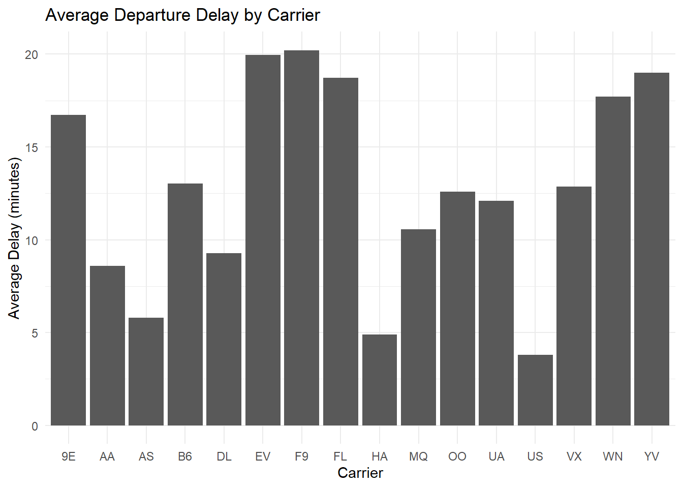
Example 70
Total number of flights each month
flights %>%
  group_by(month) %>%
  summarize(total_flights = n()) %>%
  ggplot(aes(x = month, y = total_flights)) +
  geom_line() +
  theme_minimal() +
  labs(title = "Total Flights Each Month", x = "Month", y = "Total Flights")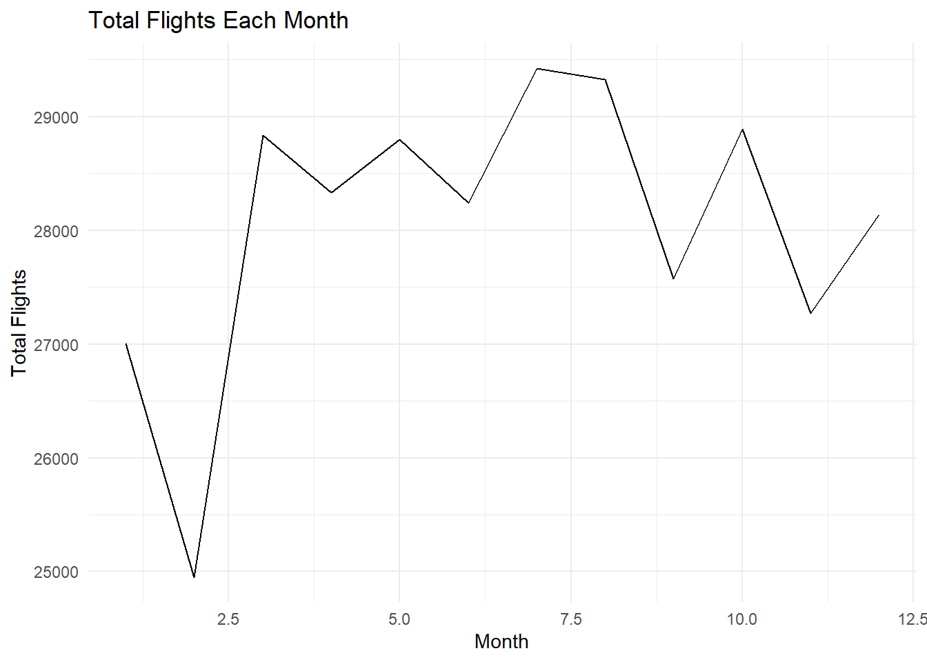
Example 71
Penguins species and their flipper length
penguins %>%
  ggplot(aes(x = species, y = flipper_length_mm, fill = species)) +
  geom_boxplot() +
  theme_minimal() +
  labs(title = "Flipper Lengths by Penguin Species", x = "Species", y = "Flipper Length (mm)")
Warning: Removed 2 rows containing non-finite values (`stat_boxplot()`).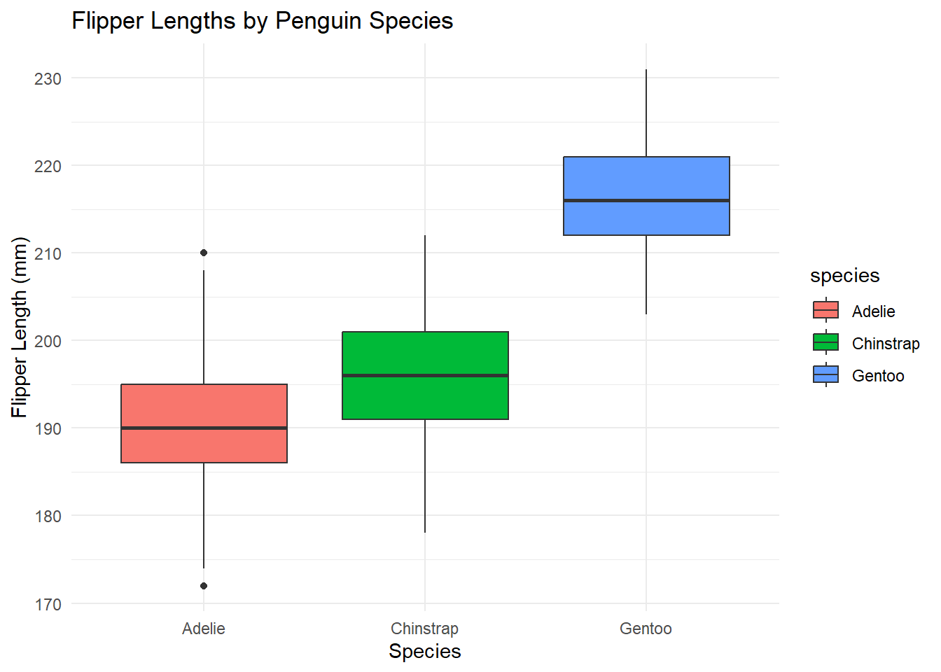
Example 72
Body mass distribution by sex for each species
penguins %>%
  ggplot(aes(x = body_mass_g, fill = sex)) +
  geom_density(alpha = 0.7) +
  facet_wrap(~species) +
  theme_minimal() +
  labs(title = "Body Mass Distribution by Sex for Each Penguin Species", x = "Body Mass (g)", y = "Density")
Warning: Removed 2 rows containing non-finite values (`stat_density()`).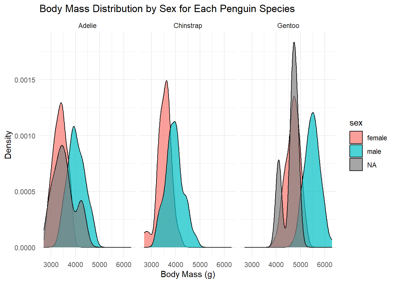
Example 73
Bill Dimensions of penguins
penguins %>%
  filter(species == "Adelie") %>%
  ggplot(aes(x = bill_length_mm, y = bill_depth_mm, color = island)) +
  geom_point() +
  theme_minimal() +
  labs(title = "Bill Dimensions of Adelie Penguins", x = "Bill Length (mm)", y = "Bill Depth (mm)")
Warning: Removed 1 rows containing missing values (`geom_point()`).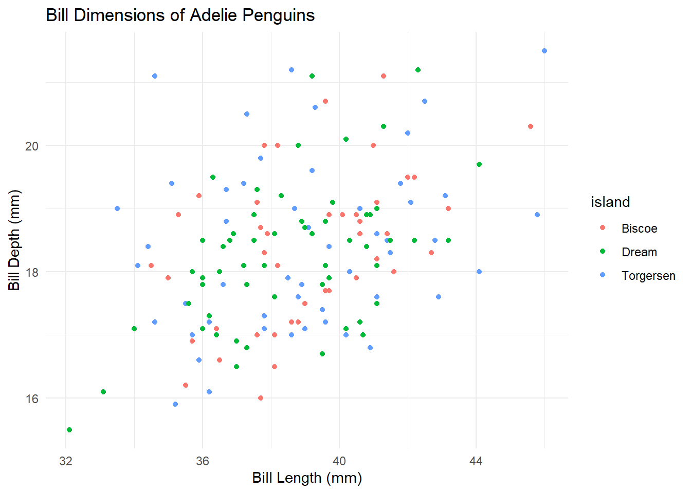
Exercise 3
1) Select the columns mpg, cyl, and gear from the mtcars dataset.
2) Filter the mtcars dataset to show only cars with 6 cylinders (cyl).
3) From the mtcars dataset, select cars with 4 gears (gear) and only display columns carb and hp.
4) Find the average miles per gallon (mpg) for each number of cylinders (cyl) in the mtcars dataset.
5) Calculate the maximum horsepower (hp) for each combination of cylinders (cyl) and gears (gear) in the mtcars dataset.
6) Add a new column disp_per_cyl to the mtcars dataset representing displacement per cylinder (calculated as disp divided by cyl).
7) Create a new column performance in the mtcars dataset, which equals “High” if mpg is greater than 20 and “Low” otherwise.
8) Create a new dataset from mtcars with only two columns: car name (row names) and miles per gallon divided by cylinders (mpg divided by cyl).
9) Arrange the mtcars dataset in descending order of weight (wt).
10) For cars with horsepower (hp) greater than 100 in the mtcars dataset, calculate the average miles per gallon (mpg), and then sort the result in descending order of this average.
11) Identify cars with an mpg less than 15 and horsepower (hp) greater than 150. Add a new column high_performance flagging them as ‘Yes’ or ‘No’.
12) Create a new column power_to_weight by dividing horsepower by weight (wt). Then find the car with the highest power_to_weight ratio.
using ‘airquality’ dataset
13) Calculate the average temperature and wind speed for each month. Add a column to show the difference in average temperature from the previous month.
14) Identify days with missing Ozone readings. Replace these missing values with the mean Ozone of that month.
using ‘swiss’ dataset
15) Categorize the Fertility rate into ‘Low’, ‘Medium’, and ‘High’ based on quantiles. Summarize the average Education level for each category.
16) Investigate the relationship between Agriculture and Examination. Create a new column Agr_Exam_Ratio (Agriculture divided by Examination) and determine which province has the highest ratio.